Alexandrou, A.^∗, Christodoulou, F., Komninos, D., Dr. Ozdeger, T., Seferis, K.

¹Blue Analytics LTD, Data Analytics and Cloud Services Provider, Nicosia, Cyprus

Received Date: December 12, 2025; Accepted Date: January 13, 2026; Published Date: January 21, 2026.

^*Corresponding author: Alexandrou A, Blue Analytics LTD, Data Analytics and Cloud Services Provider, Nicosia, Cyprus; Email: aalexandrou@blueanalytix.com

Received Date: December 26, 2025; Accepted Date: January 08, 2026; Published Date: January 17, 2026

Citation: Alexandrou A, Christodoulou F, Komninos, D, Ozdeger, T, Seferis, K (2026) Absolute Monocular Depth Estimation for Biomass Prediction in Aquaculture. Jr Aqua Mar Bio Eco: JAMBE-165

DOI: 10.37722/JAMBE.2025302

Abstract

       Accurate fish biomass estimation is essential for efficient aquaculture operations, minimizing environmental impact and reducing costs. This paper presents a monocular depth estimation system as a cost-effective alternative to traditional stereo camera setups. Our approach addresses two key challenges: (1) scaling monocular depth predictions to absolute values using regression-based models and reference object calibration, and (2) fine-tuning a state-of-the-art depth estimation model (Depth Anything v2) with stereo camera data from underwater environments. In real aquaculture cages, tile-based reference scaling—using both offline and dynamic (online) strategies—improved consistency. For fine-tuning, three model variants were trained with different maximum depth ranges. The best-performing model closely matched stereo-derived ground truth with a length error of 1.48 cm and average biomass predictions within 9%. Results demonstrate the feasibility of monocular systems for scalable, low-cost fish monitoring. While challenges remain – such as reliance on stereo data for supervision and environmental variability – our findings support the deployment of monocular depth estimation in real-world aquaculture.

Introduction

Efficient estimation of fish biomass is essential for optimizing feeding strategies, reducing operational costs, and minimizing environmental impact in aquaculture. Overfeeding leads to resource waste and water pollution due to uneaten feed, while underfeeding limits growth and reproduction. Accurate biomass estimation enables data-driven decisions that improve sustainability and profitability [1].

       Traditional biomass estimation methods often involve manually removing fish from their habitat to measure size and weight. These techniques are labor-intensive, time-consuming, and potentially harmful to fish welfare. More recently, stereo camera systems have been deployed to estimate fish dimensions and depth maps, offering improved accuracy [1] – [3]. However, stereo systems are expensive to install and maintain, particularly in large-scale or remote aquaculture facilities.

       Monocular cameras provide a promising alternative. These are often already deployed in aquaculture cages for monitoring purposes and are significantly cheaper and easier to maintain. Although monocular depth estimation models have advanced, they typically output relative depth maps, which are insufficient for tasks requiring absolute measurements—such as biomass estimation [4] – [6].

Challenges. Despite progress in monocular depth estimation, its application to underwater environments remains underexplored. Existing models struggle with generating accurate absolute depth maps [3], [7], a limitation that directly impacts the estimation of fish length and weight. Additionally, underwater imaging introduces challenges such as variable lighting, turbidity, occlusion, and noise, which further degrade model performance [8]. Depth estimation for floating or mid-water objects, such as fish, is particularly challenging because there are often no stable reference points within the scene to assist the model in inferring scale and distance [9]. This lack of contextual anchors increases prediction uncertainty, especially for objects that do not remain in fixed positions relative to the camera [10]. Furthermore, the scarcity of high-quality, labeled underwater datasets hinders effective model training and generalization [11].

       Objective and Contribution. This study aims to develop a system for estimating fish average biomass using monocular cameras, eliminating the need for costly stereo systems. Two core tasks are addressed:

1. Scaling monocular depth predictions to approximate absolute depth using regression models and reference object calibration. These methods are tested in both a controlled office setup and real aquaculture environments.
2. Fine-tuning a monocular depth estimation model using stereo camera data collected in aquaculture cages. The goal is to adapt the model to domain-specific conditions and validate its generalization across different tanks.

       Relevance and Novelty. To our knowledge, this is the first study to apply monocular depth estimation to average biomass prediction in aquaculture. By repurposing existing monocular cameras, the system offers a scalable and affordable solution for continuous fish monitoring. This approach bridges a critical gap in the field and introduces a practical method for improving aquaculture management through Artificial Intelligence (AI)-driven techniques.

Related Work

       A variety of methods have been developed for fish biomass estimation, aiming to improve upon traditional manual techniques. Li et al. [1] provide a comprehensive review of these approaches, including machine vision, acoustic methods, and environmental modeling techniques such as social network analysis (SNA). Among these, machine vision – particularly systems using stereo cameras – has shown considerable promise due to its ability to derive depth information for accurate size and weight estimation.

       Zhang et al. [3] presented a stereo-vision-based deep learning system that combines object detection with depth estimation to compute fish length and biomass with high accuracy. Similarly, another work [12] explored a deep learning pipeline for fish length estimation using stereo imagery in aquaculture tanks, demonstrating that stereo depth provides a strong foundation for accurate biomass prediction when reliable disparity maps are available.

       Feng et al. [2] proposed a binocular stereo vision method specifically applied in a breeding box environment. Similar to the previous methods, their pipeline involves underwater image enhancement to improve visibility, segmentation to isolate fish from the background, stereo matching to reconstruct 3D fish shapes, and subsequent measurement of body length.

       Besides stereo cameras, monocular camera systems offer a more cost-effective and widely deployable alternative. Yet, relative monocular depth prediction remains challenging. Monocular depth estimation models inherently predict relative depth values, which lack a consistent metric scale across scenes. For applications such as fish biomass estimation, this limitation must be addressed by converting these relative maps into metric-scale depth. Masoumian et al. [13] proposed a hybrid framework that couples monocular depth estimation (via a custom autoencoder) with object detection using YOLOv5. Their key innovation lies in introducing reference objects of known size within the scene and collecting their corresponding monocular and stereo-derived depth values. Using these paired measurements, they fit polynomial regression models (linear, quadratic, and cubic) to derive a scaling function:

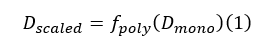
where f_poly represents the learned polynomial mapping from monocular to stereo depth. This allowed the relative monocular predictions to be transformed into absolute depth maps suitable for precise geometric measurements.

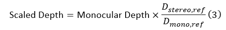
       Mei et al. [14] introduced a non-learning-based calibration technique that requires only sparse, accurate depth samples within the target environment. These sparse measurements can come from low-cost rangefinders, stereo snapshots, or known scene geometry. The method computes a global scale factor and bias by minimizing the discrepancy between the sparse ground truth depths and the relative depth values predicted by a foundation model:

where s and b are computed via least-squares fitting. This approach avoids re-training the depth network entirely, enabling rapid deployment in new environments.

       Another work [15] tackled the problem of underwater metric depth estimation by building a real-world benchmark dataset containing paired RGB and ground truth depth maps captured in diverse aquatic conditions. Their experiments revealed that monocular models trained on terrestrial datasets suffer significant performance drops underwater due to domain shift. To address this, they proposed synthetic domain adaptation: generating large-scale, photorealistic underwater imagery with corresponding depth maps, and fine-tuning terrestrial models on this synthetic data. This process significantly improved the models’ ability to predict metric depth in real underwater scenes.

       Furthermore, depth models such as Depth Anything V2 [16] offer absolute depth-map estimation. Yang et al. [16] developed Depth Anything V2, a general-purpose monocular absolute depth estimation model pre-trained on billions of pseudo-labeled real-world images. The model uses large-scale self-supervision with metric depth annotations from diverse sources to learn scale-aware depth features. When fine-tuned on domain-specific datasets – such as underwater aquaculture imagery – it adapts to the target domain while preserving metric accuracy. This enables monocular systems to achieve near-stereo performance for absolute depth estimation without explicit reference objects in the scene. Other similar depth models are SharpDepth [17], Depth Pro [18], Metric3D v2 [19].

       Despite the progress of these state-of-the-art methods, several limitations remain that restrict their deployment in real aquaculture settings. Stereo-based approaches, while accurate, depend on costly and logistically complex hardware installations. Furthermore, many existing studies are conducted in controlled environments such as breeding boxes or longline chutes, where assumptions about fish orientation or fixed reference planes simplify calibration. However, these assumptions rarely hold in large-scale open-sea cages, where fish move freely in three dimensions under variable lighting, turbidity, and occlusion. Methods relying on many reference objects or sparse external measurements introduce practical constraints, as such objects may not always be present or accessible in dynamic underwater environments. Furthermore, many monocular depth models struggle with domain shifts, particularly when transferring from terrestrial to underwater imagery, often requiring extensive synthetic fine-tuning to regain accuracy. Even the latest foundation models such as Depth Anything V2 or Depth Pro, though capable of producing absolute depth without explicit scaling, demand careful domain adaptation and substantial computational resources. These gaps highlight the need for solutions that are cost efficient, flexible in deployment, and robust to underwater variability.

Materials And Methods

A. Overview

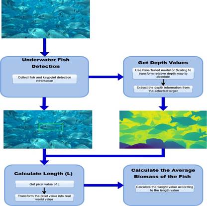
       This work addresses the challenge of accurate biomass estimation using monocular depth estimation in underwater aquaculture environments. The methodology is divided into two primary tasks: 1) Scaling Monocular Depth and 2) Fine-tuning a Monocular Depth Model.

       The overall pipeline for length and average biomass prediction is illustrated in Figure 1.

       B. Experimental Materials: Hardware and Software Components

The experiments were conducted in Greece within aquaculture cages containing approximately 400,000 fish per cage. The following hardware and software components were employed to support both the depth scaling and model fine-tuning tasks.

1. Camera System: A commercial stereo vision camera was utilized, equipped with integrated functionality for generating dense depth maps and 3D point clouds alongside RGB video, recording at HD resolution and 30 FPS. For underwater use, the stereo camera was enclosed in a waterproof housing. This prototype stereo camera system was used to generate monocular RGB frames and corresponding ground truth depth maps, forming the baseline for performance evaluation of the proposed methodology.
2. Reference Objects: Reference objects played a key role in calibration and scaling. A dummy fish of known length (30 cm) was used in both office and underwater experiments for length and depth estimation validation. Additionally, a rigid 10×10 cm flat tile was mounted in front of the stereo camera on an aluminium bracket for underwater scaling experiments. This tile served as a fixed reference for deriving scaling formulas and calibrating monocular depth maps.
3. Computing Hardware: A workstation equipped with an NVIDIA RTX 3090 GPU, Intel Core i7 CPU, 32 GB of RAM, and a 1 TB SSD was used to handle deep learning model training, scaling experiments, and real-time video processing.
4. Deep Learning Model: Depth-Anything-V2Small [16] was selected for its balance between accuracy and computational efficiency. The model contains 24.8M parameters and is optimized for efficient monocular depth estimation. Depth Anything V2 is one of the most recent monocular depth estimation models, achieving state-of-the-art performance across multiple benchmarks. In addition, it provides publicly available scripts for fine-tuning, supports varied model sizes (Small, Base, Large), and is trained on billions of pseudo-labelled images, making it highly adaptable to new domains.

C. Data Description

1. Data Sources: Data were collected from both controlled office (air) environments and operational aquaculture cages in Greece. These datasets supported the development and evaluation of both the scaling and fine-tuning methodologies.
2. Data Collection: For office-based experiments, 100 stereo camera frames were captured, containing multiple objects. Approximately 80% of the frames were used to annotate around 1,000 stereo-monocular point pairs for training regression models.

In the aquaculture environment, 50 frames were extracted featuring a reference tile affixed to the camera. These were used for offline scaling calibration by collecting 500 annotated depth points. Online scaling was performed dynamically during real-time video processing using the same tile, without collecting additional data.

       For evaluation, 10,000 test frames were extracted from stereo footage of an aquaculture cage and used to benchmark scaling accuracy.

       To train and validate the fine-tuned monocular depth model, approximately 45,000 camera frames with corresponding depth maps were collected. 80% of this data was used for training and 20% for validation. Additional 15,000 frames from the same cage were reserved for testing the generalization performance of the fine-tuned model.

       To minimize the influence of environmental variability on depth estimation, image acquisition in aquaculture cages was conducted during stable daylight conditions and under moderate water clarity. The camera was positioned at consistent depth and orientation across sessions to ensure repeatable lighting geometry. Whenever turbidity increased significantly, recording was paused until visibility stabilized. No artificial lighting was used; instead, automatic exposure and white balance correction were enabled in the stereo camera, to normalize brightness and color variations across frames. These precautions helped ensure that differences in water clarity, lighting, and particle density did not bias the depth estimation process.

• Data Preprocessing: Minimal preprocessing was applied to the scaling data. For the fine-tuning task, RGB images and depth maps were resized to 518 × 518 pixels. Input images were normalized using ImageNet statistics (mean: [0.485, 0.456, 0.406]; std: [0.229, 0.224, 0.225]). Data augmentation included random cropping and horizontal flipping to simulate varied viewpoints. Color-based augmentation was excluded, as it did not improve training performance in the underwater domain.

D. Task 1: Scaling Monocular Depth Estimation

1. Approach 1 – Office Experiments: To test the feasibility of scaling monocular depth predictions to absolute measurements, a controlled experiment was conducted in an office (air) environment. The stereo camera was mounted on a table, and a set of reference objects was placed at different known distances and orientations. Depth maps were extracted from the stereo camera and from the monocular model (Depth Anything V2). Corresponding points on the reference objects were manually annotated (typically 8 – 10 samples per object and per frame), providing paired monocular and stereo depth values across different scene depths. These point pairs were used to compute a scaling factor and to fit Linear, Quadratic, and Cubic polynomial regression models. A single-object scaling strategy was also tested by computing a global scaling factor using one reference object only.

In all cases, monocular depth values were transformed into metric depth using the general scaling equation:

Here D_{stereo, ref} and D_{mono, ref} represent the average stereo and monocular depth values of the annotated reference points, respectively. The regression-based models extend this general formulation by learning a polynomial mapping from D_mono to D_stereo using all annotated pairs.

• Approach 2 – Underwater Experiments (Tile Scaling): To evaluate monocular scaling in real aquaculture conditions, experiments were conducted in a submerged cage housing approximately 400,000 fish. A tile was securely mounted in front of the stereo camera and used as a visual reference object. Depth frames were recorded under varying underwater lighting and turbidity conditions. The tile provided a known physical scale within the scene, enabling calibration of monocular depth maps using both offline and online strategies. For these experiments, the same transformation (Equation (3)) was used. The only difference lies in how the reference depth terms

(Dstereo, ref and Dmono, ref) were obtained.

1. Offline Scaling: In the offline approach, 50 frames containing the tile were extracted from stereo camera footage. For each frame, the tile’s pixel location was predefined. Average depth values for the tile were calculated from both the monocular and stereo depth maps.
2. Online Scaling: The online approach dynamically estimated the scaling factor during video processing. In each frame, the region containing the tile was cropped, and its average depth from the monocular map was computed in real time. A frame-filtering mechanism was implemented to exclude frames where the tile was occluded or the depth fell outside a valid range (530–540 mm), based on the distribution of stereo-derived tile depths observed offline.

For both scaling approaches, fish and keypoint detection were then applied to obtain mouth and tail locations, from which 3D standard fish length (L) and biomass were computed using the scaled monocular depth. Additionally, prediction errors were analyzed across different predicted depth bins to identify performance trends.

E. Task 2: Fine-Tuning the Monocular Model

       The second task focused on adapting the Depth Anything V2 model [16] to the underwater aquaculture environment through supervised fine-tuning. The objective was to improve the model’s ability to predict accurate depth maps under challenging conditions such as noise, occlusion, and lighting variability.

       Three variants of the Depth Anything V2 Small model were trained using paired RGB images and stereo-derived depth maps:

• Model v1: Trained on full-frame depth maps with a maximum depth of 5 meters (baseline).
• Model v2: Trained with a depth cap of 1 meter, focusing on foreground fish.
• Model v3: Trained with a depth cap of 2 meters, allowing a broader depth range.

       Each model was initialized with pre-trained encoder weights. The decoder was randomly initialized and trained to adapt specifically to the aquaculture domain.

The best-performing model was further tested across different aquaculture cages to assess generalization to unseen environments. Length, depth, and biomass predictions were compared against stereo-derived ground truth.

F. Length and Biomass Estimation

Standard length (L) was computed by identifying two keypoints either manually or using a detection model (e.g., Faster R-CNN) [20]. The pixel coordinates were converted to 3D real-world coordinates using the scaled depth map and camera intrinsics:

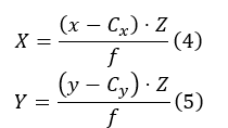
where (x, y) are pixel locations, Z is the depth, C_x, C_y  are

the principal points, and f is the focal length. The length (L) in 3D space was computed using the

Euclidean distance:

The estimation of biomass (W) from length (L) follows the well-established length–weight relationship (LWR) [21]:

The values for a, b were estimated on our dataset and found to align well with the typical values for Sparus aurata (gilthead seabream, locally “tsipoura”).

G. Evaluation Metrics

       All models and scaling methods were evaluated based on their ability to accurately estimate depth, length (L), and biomass. The evaluation was carried out in direct comparison with the stereo camera results, which were assumed as ground truth. The following metrics were used consistently across all experiments:

• Mean Absolute Error (MAE): Measures the average magnitude of absolute errors between predictions and ground truth.

where   is the predicted value,  is the ground truth, and N is the number of samples.

• Standard Deviation (STD): Measures the dispersion of absolute errors to evaluate consistency.

• Biomass Accuracy: The average predicted biomass was compared to the average ground truth biomass:

where  is the predicted biomass and  is the true biomass derived from stereo length estimates.

IV. RESULTS

A. Task 1 – Scaling Monocular Depth Estimation

1)            Approach 1: Office Experiments: Three regression models—linear, quadratic, and cubic—were trained to scale monocular depth predictions to match stereo-derived ground truth. Table I shows their performance based on R² and MSE scores.

Τable Ι

Performance of Polynomial Regression Models for Depth Scaling (Office Environment).

Model	R2	MSE (mm2)
Linear Regression	0.981	56.42
Quadratic Regression	0.988	41.85
Cubic Regression	0.994	22.17

       The cubic regression model achieved the best fit, outperforming the linear and quadratic models.

       Using the scaled depth predictions from the cubic model, length (L) was computed for a dummy fish object placed at various depths and orientations. The L estimation results are shown in Table II.

       The results demonstrate high length accuracy (under 5 mm MAE) and consistent biomass predictions.

Table ΙΙ

Regression Model	Mean Monoscopic L (cm)	Std Monoscopic L (cm)	Mean L Error (cm)	L MAE (cm)	L Error STD (cm)
Linear	28.76	3.13	1.42	3.55	2.08
Quadratic	28.41	3.05	1.48	3.23	1.75
Cubic	29.85	1.93	0.46	1.78	1.85
Single object	29.75	3.18	0.56	3.12	1.68

Evaluation L Results: Office Environment

a)            Generalization to Real Environment: The cubic regression model was also applied to monocular frames from a real aquaculture cage. However, accuracy decreased due to underwater variability (Table III).

Table ΙΙI

Biomass and L Prediction Results: Aquaculture Environment

Regression Model	Predicted Average Biomass (g)	Predicted Average L (cm)	Predicted L STD (cm)
Linear	705.63	28.86	5.12
Quadratic	708.86	28.90	5.06
Cubic	646.26	28.07	5.73
Single object	689.23	28.64	5.39
Ground Truth	421.58	24.52	2.33

2)            Approach 2: Underwater Experiments (Tile Scaling):

1. Scaling Formulas: For both offline and online methods, depth scaling was performed using Equation (1). In the offline case, the scaling factor was computed from pre-annotated averages:

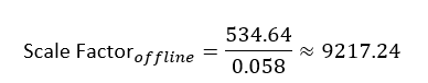
For online scaling, the numerator remained constant at 534.64 mm (average stereo tile depth), but the denominator – the monocular tile depth – was estimated per frame in real-time:

• Comparison of Scaling Methods: The average predictions for L and biomass, along with L variability, are shown in Table IV.

Τable ΙV

L and Average Biomass Predictions in Aquaculture Environment.

Method	Avg. Biomass (g)	Avg. L (cm)	L STD (cm)
Offline Scaling	500.94	25.90	3.09
Online Scaling	471.00	25.40	3.95
Ground Truth	392.82	23.98	2.39

       Offline scaling achieved closer estimates to the true average L and biomass. Online scaling produced more variable results but adapted better to real-time environmental changes.

Table V

L and Depth Prediction Errors.

Method	L MAE (cm)	L STD (cm)	Depth MAE (mm)	Depth STD (mm)
Offline Scaling	3.01	3.13	8.14	8.39
Online Scaling	3.45	2.57	9.20	7.07

• Depth and L Errors: Table V shows the L and depth errors for both approaches.

While offline scaling offered slightly lower average errors, the online method had more stable error distribution (lower STD).

• Error Trends Across Depth Ranges: To better understand performance across different distances, we analyzed L and depth MAE as a function of predicted depth bins. Figures 2 and 3 illustrate this relationship.

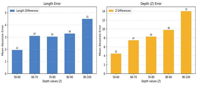
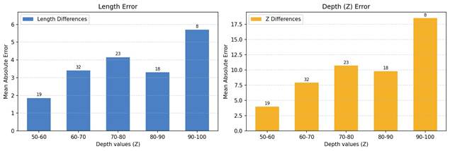
       Both methods exhibited increasing error at greater predicted depths, confirming the reduced reliability of monocular estimation at longer ranges.

To mitigate this issue, predictions with estimated depths greater than 90 cm were excluded. Table VI shows the results after filtering.

Table VI

L and Depth Errors After Filtering Out Predictions with Depth Greater Than 90 Cm.

Method	L MAE (cm)	L STD (cm)	Depth MAE (mm)	Depth STD (mm)
Offline Scaling	2.76	2.97	6.84	7.26
Online Scaling	3.19	2.56	7.65	6.17

Filtering out distant fish improved accuracy across both methods, confirming the benefit of discarding unreliable long-range predictions.

B. Task 2 – Fine-Tuning the Monocular Model

1. Training and Validation Performance: Three variants of the Depth Anything V2 model were fine-tuned using stereo derived ground truth from underwater scenes, with varying maximum depth caps. Table VII summarizes their training losses and validation metrics.

Τable VII

model	max depth (m)	loss	d1	AbsRel	RMSE	SILog
Model v1	5 (baseline)	0.22	0.76	0.16	0.44	0.25
Model v2	1	0.09	0.92	0.09	0.091	0.13
Model v3	2	0.15	0.83	0.13	0.19	0.19

Training and Validation Metrics for Fine-Tuned Models.

       Model v2 achieved the best overall validation performance across all metrics. In contrast, Model v1 showed the weakest results, indicating that limiting the maximum depth improves the focus on foreground fish and reduces overall error.

• L and average Biomass Estimation Accuracy: Table VIII presents the average L and biomass predictions from each model compared with ground truth values.

Table VIII

L and Average Biomass Prediction Accuracy of Fine-Tuned Models.

Model	Avg. Biomass (g)	L (cm)	L STD (cm)
Model v1	440.02	24.86	3.06
Model v2	358.14	23.29	4.89
Model v3	475.46	25.47	3.05
Ground Truth	392.82	23.98	2.39

Model v2 produced L and average biomass values closest to ground truth, while Model v1 and Model v3 overestimated both metrics.

• Depth and L Error Analysis: Table IX presents absolute errors and standard deviations for depth and L predictions.

Table IX

Depth and L Prediction Errors for Fine-Tuned Models.

Model	L MAE (cm)	L STD (cm)	Depth MAE (cm)	Depth STD (cm)
Model v1	1.84	1.22	4.84	3.80
Model v2	1.48	1.08	3.94	3.06
Model v3	1.53	1.06	3.99	3.05

Model v2 again demonstrated the lowest average errors, reinforcing its effectiveness for underwater biomass estimation.

• Error Trends by Depth Range: Mean absolute errors for L and depth were analyzed across different predicted depth bins. After filtering out predictions with depth greater than 90 cm, error metrics improved for all models (Table X).

Filtering depth outliers substantially reduced both L and depth error, confirming that monocular models remain most reliable within a foreground range (≤ 90 cm).

Table X

L and Depth Errors for Predictions Less Than 90 cm.

Model	L MAE (cm)	L STD (cm)	Depth MAE (cm)	Depth STD (cm)
Model v1	1.74	1.13	4.23	2.86
Model v2	1.45	1.03	3.52	2.50
Model v3	1.51	1.02	3.72	2.56

e)            Generalization to Unseen Cages: Model v2 was tested on videos from five different aquaculture cages. Table XI compares predicted L values to ground truth for each case.

Table XI

Model v2 L Predictions on Unseen Cages.

Test Set	Predicted L (cm)	Ground Truth L (cm)	L Error (cm)
PRX05	23.29	23.98	0.69
Cage 15p	26.30	25.16	1.14
Cage 11p	25.18	24.91	0.27
Cage M7	24.74	24.61	0.13
Cage M10	24.06	25.43	1.37

Model v2 demonstrated good generalization across cages, with L error remaining under 1.4 cm in all cases.

Discussion

A. Interpretation of Results

1)            Approach 1 – Office Experiments: The office experiments confirmed the feasibility of scaling monocular depth predictions into absolute values using regression techniques, within a specific domain. Among the tested models, cubic regression yielded the best performance with an R² of 0.99 and MSE of 307.09, outperforming linear and quadratic alternatives. This indicates that depth prediction relationships are inherently non-linear and benefit from higher-order polynomial fitting.

       L estimation results followed a similar trend. The cubic model achieved the lowest L MAE (1.78 cm) and L error STD (1.93 cm), demonstrating its robustness in length prediction. The cubic model accurately predicted L by generalizing learned object-scale relationships. In contrast, linear and quadratic models showed higher error variances, indicating limited expressiveness for underwater complexity.

       Interestingly, a single-object scaling method based on a known reference object produced comparable results (L MAE = 3.12 cm), further suggesting that simplified scaling techniques can still be viable in controlled environments.

       However, when applied in aquaculture test environments, all scaling models underperformed significantly. The cubic model, though still best among them, predicted an inflated average L of 28.1 cm (vs. ground truth 24.5 cm), and L STD rose to 5.73 cm, indicating reduced reliability. This degradation illustrates the environment-specific nature of regression scaling and highlights the need for adaptive recalibration in real-world settings.

• Approach 2 – Underwater Experiments (Tile Scaling): The underwater tile experiments revealed that using a physical reference object to scale monocular depth maps can significantly improve performance in dynamic environments. Both offline and online scaling methods predicted average Ls within 1.9 cm of the ground truth (23.98 cm), with offline achieving slightly higher consistency (L STD = 3.09 cm).

In terms of error, offline scaling achieved lower L MAE(3.01 cm) and depth MAE (8.14 cm) compared to online

(3.45 cm and 9.20 cm, respectively). However, online scaling delivered lower L and depth error STD with 2.57 cm and 7.07 cm respectively, suggesting that dynamic adaptation offered better frame-by-frame consistency under variable conditions.

Further error stratification by predicted depth bins revealed that both approaches suffer increased inaccuracies at larger depth predictions. Filtering predictions above 90 cm improved L and depth errors in both cases – offline L MAE dropped to 2.76 cm and depth MAE to 6.84 cm – confirming that monocular models are most effective at close-to-mid range depths.

• Task 2 – Fine-Tuning the Monocular Model: Finetuning the Depth Anything V2 model for aquaculture domains significantly improved performance. Model v2 (max depth = 1 meter) achieved the best results across all metrics: AbsRel (0.09), RMSE (0.091), SILog (0.13), and L MAE (1.48 cm). Its superior performance illustrates how restricting the prediction range to foreground depths (0 – 1 m) enhances the model’s precision in targeting fish-specific features while minimizing noise from distant objects.

This depth-constrained fine-tuning not only improved accuracy in the training domain but also demonstrated strong generalization. On unseen cages, Model v2 maintained low L errors (e.g., 0.13 – 1.37 cm), indicating domain transferability within similar environmental conditions.

       Visual inspection (Figure 4) supported these findings, where Model v2 predictions most closely aligned with stereo-derived depth maps and successfully ignored irrelevant background information.

       Error filtering for predictions below 90 cm further boosted performance, but slightly. Model v2’s filtered L MAE improved from 1.48 to 1.45 cm and depth MAE from 3.94 to 3.52 cm. Although the benefit was minimal, constraining predictions to ranges where monocular models are most effective can still be beneficial when fine-tuning the model.

       In conclusion, the results clearly demonstrate that domain adaptive fine-tuning, especially with targeted depth constraints, provides the most accurate and generalizable solution for monocular biomass estimation in aquaculture settings.

B. Integration into Real-Time Monitoring Systems

       The proposed monocular depth estimation framework can be readily integrated into automated aquaculture monitoring systems. Since the model operates on single RGB frames, it can process continuous video streams from low-cost underwater cameras in real time using edge devices equipped with moderate GPUs. The system can automatically estimate standard fish length and biomass without human intervention, providing continuous growth tracking and feeding optimization. Integration with existing farm management software infrastructures would allow remote visualization and data logging, enabling farmers to make data-driven decisions.

C. Implications for Aquaculture

       The findings of this study carry several practical implications for aquaculture operations, particularly in enhancing the accessibility and efficiency of fish biomass estimation. By leveraging monocular cameras – which are typically already deployed in aquaculture systems – farmers can repurpose existing infrastructure without the need for costly and complex stereo setups. Stereo cameras can instead be reserved for periodic calibration or data collection.

       Monocular cameras offer significant cost advantages, being more affordable, compact, and easier to maintain than stereo systems. This low barrier to entry makes technology accessible not only to large-scale fish farms but also to smaller enterprises seeking to optimize feeding strategies.

       Improved feeding decisions enabled by accurate biomass estimation can reduce feed waste, lower operational costs, and mitigate environmental impacts such as water pollution caused by overfeeding. Additionally, eliminating the need for manual fish handling minimizes stress on fish populations, promoting better growth rates and welfare. Overall, the integration of AI-driven monocular depth estimation offers a scalable and sustainable solution for modern aquaculture.

D. Limitations and Open Challenges

       Despite the promising results, several limitations must be acknowledged. The most significant challenge lies in the reliance on stereo camera data for supervision. Although these cameras are used as ground truth providers, they are not immune to depth estimation errors, especially in turbid or poorly lit underwater environments. As a result, the fine-tuned monocular model may learn from imperfect labels.

Furthermore, stereo cameras may not be deployable in every aquaculture cage, particularly in remote or inaccessible locations, limiting the generalization of fine-tuned models. While the fine-tuning approach showed robust results under specific conditions, its performance under more extreme underwater variability – such as significant changes in water clarity, light diffusion, or dense fish occlusion – remains untested.

       Another critical constraint is that monocular depth models inherently predict relative depth. Even after fine-tuning, the depth maps remain sensitive to scene composition and lighting conditions, and their predictions may be unreliable in some operational scenarios without continuous recalibration or filtering mechanisms.

Finally, it is important to note that the fine-tuned model was evaluated using the left view of the stereo camera rather than an independent monocular camera. As a result, the camera characteristics (e.g., resolution, intrinsic parameters, optical quality) of the test input were identical to those used for training. In real-world deployments, monocular cameras may differ significantly in terms of sensor specifications and image quality, which could lead to a drop in performance if the model is applied without further calibration or adaptation.

E. Future Work

       Several avenues for future research can be explored to further enhance the robustness and generalizability of monocular depth estimation systems for aquaculture. First, expanding the training dataset to include images collected from a wider range of aquaculture environments – encompassing different cages, fish species, size distributions, and environmental conditions – would substantially enhance the model’s generalization capability and mitigate overfitting. Moreover, accounting for variations in fish morphology, water turbidity, and lighting conditions across pond, tank, and open-sea systems is essential to ensure robust and accurate depth estimation under diverse real-world scenarios.

       Additionally, future scaling experiments could include more than one reference object inside the aquaculture environment (e.g., multiple tiles at different locations) in order to obtain a more stable and accurate scaling factor. Furthermore, extensive testing across different cages would also be beneficial. A larger set of test scenarios – including cages with different lighting conditions, water clarity levels, and fish densities – would allow both the scaling and fine-tuning approaches to be evaluated under more realistic and diverse operational settings.

       It would also be useful to benchmark the proposed method against other recent monocular depth models (e.g., Apple’s Depth Pro [18]), in order to evaluate whether newer architectures can provide better baseline accuracy or generalization.

       Another promising direction consists of using explicit foreground masks (i.e., fish only) during training instead of generic depth thresholds. This could encourage the model to focus more specifically on fish contours and shapes, potentially yielding more precise predictions. Further improvements might also be achieved by training high-capacity versions of the Depth Anything V2 model that are able to capture more complex spatial relationships within the scenes.

       Finally, since the current fine-tuning experiments were carried out using one view of the stereo camera, it will be important to validate the approach using actual monocular cameras. This will verify whether the proposed method still yields reliable results when applied to real-world monocular input with potentially different sensor properties.

Conclusion

This study proposed a practical and cost-effective approach to fish average biomass estimation using monocular depth estimation techniques tailored for aquaculture environments. Two complementary strategies were explored: scaling monocular depth maps using regression and reference-based techniques, and domain-specific fine-tuning of a monocular depth estimation model. While regression-based scaling worked well in controlled office settings, its accuracy degraded in real aquaculture environments, emphasizing the need for adaptive calibration.

       Tile-based scaling showed better performance underwater, with offline and online methods offering complementary strengths. However, it was the fine-tuning of the Depth Anything V2 model that delivered the most promising results, achieving high accuracy in length and average biomass prediction and showing generalization across different cages when constrained to foreground depths.

       The study demonstrates that monocular cameras – when paired with AI and appropriate calibration – can rival stereo systems in accuracy while offering greater scalability and affordability. These findings pave the way for a more accessible and sustainable future in aquaculture monitoring, where intelligent visual systems empower farmers to optimize productivity and environmental stewardship.

Data Availability

       The dataset used in this study was collected on-site in commercial aquaculture cages and is therefore proprietary, subject to data ownership and privacy agreements with the farm operator. As such, it is not publicly available.

Declaration

       All imaging procedures described in this study were noninvasive and did not involve the physical handling of fish. Data collection was carried out with the full consent of the farm operators and in accordance with established aquaculture welfare guidelines. The experiments were designed to ensure minimal disturbance to the fish and full compliance with animal welfare standards.

Acknowledgements

       This work has received funding via the Next Generation EU Restart 2016–2020 Programme, project ID ENTERPRISES/0223/Sub-Call1/0157.

References

1. Li, Y. Hao, and Y. Duan, “Nonintrusive methods for biomass estimation in aquaculture with emphasis on fish: A review,” Reviews in Aquaculture, vol. 12, no. 3, pp. 1390–1411, 2020.
2. G. Feng, B. Pan, and M. Chen, “Non-Contact Tilapia Mass Estimation Method Based on Underwater Binocular Vision,” Applied Sciences, vol. 14, no. 10, p. 4009, Jan. 2024.
3. T. Zhang, Y. Yang, Y. Liu, C. Liu, R. Zhao, D. Li, and C. Shi, “Fully automatic system for fish biomass estimation based on deep neural network,” Ecological Informatics, vol. 79, p. 102399, 2024.
4. C. Zhang, X. Weng, Y. Cao, and M. Ding, “Monocular Absolute Depth Estimation from Motion for Small Unmanned Aerial Vehicles by Geometry-Based Scale Recovery,” Sensors, vol. 24, no. 14, p. 4541, Jan. 2024.
5. F. Xue, G. Zhuo, Z. Huang, W. Fu, Z. Wu, and M. H. A. Jr, “Toward Hierarchical Self-Supervised Monocular Absolute Depth Estimation for Autonomous Driving Applications,” Sep. 2020.
6. R. Fan, T. Ma, Z. Li, N. An, and J. Cheng, “Region-aware Depth Scale Adaptation with Sparse Measurements,” Jul. 2025.
7. D. Suhoi, “Metric and relative monocular depth estimation: An overview. fine-tuning depth anything v2,” https://huggingface.co/blog/Isayoften/ monocular-depth-estimation-guide, Feb. 2025, a blog post on Hugging Face.
8. X. Yang, X. Zhang, N. Wang, G. Xin, and W. Hu, “Underwater selfsupervised depth estimation,” Neurocomputing, vol. 514, pp. 362–373, Dec. 2022.
9. P. Agand, M. Chang, and M. Chen, “DMODE: Differential Monocular Object Distance Estimation Module without Class Specific Information,” May 2024.
10. H. Hu, Y. Feng, D. Li, S. Zhang, and H. Zhao, “Monocular Depth Estimation via Self-Supervised Self-Distillation,” Sensors (Basel, Switzerland), vol. 24, no. 13, p. 4090, Jun. 2024.
11. J. Er, J. Chen, Y. Zhang, and W. Gao, “Research Challenges, Recent Advances, and Popular Datasets in Deep Learning-Based Underwater Marine Object Detection: A Review,” Sensors, vol. 23, no. 4, p. 1990, Jan. 2023.
12. Tonachella, A. Martini, M. Martinoli, D. Pulcini, A. Romano, and F. Capoccioni, “An affordable and easy-to-use tool for automatic fish length and weight estimation in mariculture,” Scientific Reports, vol. 12, no. 1, p. 15642, Sep. 2022.
13. Masoumian, D. G. F. Marei, S. Abdulwahab, J. Cristiano, D. Puig, and H. A. Rashwan, “Absolute distance prediction based on deep learning object detection and monocular depth estimation models,” Oct. 2021.
14. J. Mei, J.-N. Hwang, S. Romain, C. Rose, B. Moore, and K. Magrane, “Absolute 3d pose estimation and length measurement of severely deformed fish from monocular videos in longline fishing,” 2021.
15. [Online]. Available: https://arxiv.org/abs/2102.04639
16. H. Liu, M. Roznere, and A. Q. Li, “Deep Underwater Monocular Depth Estimation with Single-Beam Echosounder,” in 2023 IEEE International Conference on Robotics and Automation (ICRA). London, United Kingdom: IEEE, May 2023, pp. 1090–1097.
17. L. Yang, B. Kang, Z. Huang, Z. Zhao, X. Xu, J. Feng, and H. Zhao, “Depth Anything V2,” Oct. 2024.
18. D.-H. Pham, T. Do, P. Nguyen, B.-S. Hua, K. Nguyen, and R. Nguyen, “Sharpdepth: Sharpening metric depth predictions using diffusion distillation,” in Proceedings of the IEEE/CVF Conference on Computer Vision and Pattern Recognition (CVPR), June 2025, pp. 17060–17069.
19. Bochkovskii, A. Delaunoy, H. Germain, M. Santos, Y. Zhou, S. R. Richter, and V. Koltun, “Depth Pro: Sharp Monocular Metric Depth in Less Than a Second,” Apr. 2025.
20. M. Hu, W. Yin, C. Zhang, Z. Cai, X. Long, K. Wang, H. Chen, G. Yu, C. Shen, and S. Shen, “Metric3Dv2: A Versatile Monocular Geometric
21. Foundation Model for Zero-shot Metric Depth and Surface Normal Estimation,” IEEE Transactions on Pattern Analysis and Machine Intelligence, vol. 46, no. 12, pp. 10579–10596, Dec. 2024.
22. S. Ren, K. He, R. Girshick, and J. Sun, “Faster R-CNN: Towards RealTime Object Detection with Region Proposal Networks,” Jan. 2016.
23. N. Jisr, G. Younes, C. Sukhn, and M. H. El-Dakdouki, “Length-weight relationships and relative condition factor of fish inhabiting the marine area of the Eastern Mediterranean city, Tripoli-Lebanon,” Egyptian Journal of Aquatic Research, vol. 44, no. 4, pp. 299–305, 2018.