Evaluation of pollution risks level in Thar-Jath oilfields South Sudan
Bior J A*1,2, 1FozaoK F1, Tsamo C3, Suh C E4
*Corresponding author: BIOR JAMES AKOI, The University of Bamenda-Cameroon North-west Region, Cameroon. Email: juniorbior25@gmail.com
Citation: Bior J A, Fozao K F, Tsamo C, Suh C E (2025) Evaluation of pollution risks level in Thar-Jath oilfields South Sudan. Adv Agri Horti and Ento: AAHE-227
DOI: 10.37722/AAHAE.2025204
Watch the Article in Motion
Abstract
The study was carry out to assess the pollution, impact, and risk level to the surface water environment of pollutants in the water bodies of Thar-jath Unity State South Sudan. The parameters for evaluating surface water quality and risks included temperature, pH, TSS, BOD, COD, NH4+-N, NO2–-N, NO3– -N, PO43- -P, Cl–, Fe, and coliform. Surface water samples were collect at different locations with a frequency of five times (March. April. May, June, and August) in 2024. The water quality index (WQI), impact and risk level (risk quotient or RQ, RQ-F), correlation analysis, and principal component analysis (PCA) were utilize in the study. The results show that the surface water have been seriously polluted due to organic matter, nutrients, microorganisms, iron, and salinity. The values of WQI in the dry and rainy seasons fluctuated between bad and very good, indicating that surface water quality is suitable for water transport and other purposes with higher quality requirements. TSS, COD, Fet and coliform have a high impact and risk for the environment in this study area. There were no environmental impacts and risks to NO3–-N. Locations with many high-risk pollutants were mainly distribute in river side and production areas. The significant negative correlation between the WQI and RQ indicated that the lower the WQI, the higher the environmental risk. The PCA results show that at least six polluting sources affected water quality and caused environmental risks. The results of this study contribute essential and valuable information for improving water quality in the study area through the assessment of environmental impacts and risks.
Keywords: Pollutants, Principal component analysis, Pearson correlation, Risk levels, Surface Water Bodies
Introduction
Petroleum is one of the most important resources in the world. Oilfield drilling and exploitation distribute widely in the area where oil have been extract. The oilfield drilling sites are generally consider as the multiple-point sources of contamination to surface water. Pollution in surface water incidents occur frequently in oil exploitation, transportation, and processing Wang W et al. (2014). Oil leakage in the process of oil recovery would produce great harm to surface water quality, especially carcinogenic, teratogenic, and mutagenic petroleum pollutants Wang W et al. (2014). They are greatly harmful to the ecological environment and human health Miao Y et al. (2016). It is essential to evaluate oil-drilling hazards to the environment, especially to surface water. Therefore, the surface water pollution risks assessment is strongly necessary in this area. Surface water risk assessment is an essential tool for prevention and control of oil leakage An Y et al. (2016); Sun X (2014). It is highly associated with ecological, agricultural, industrial, and human activities. According to Kaliraj S et al. (2015), the influence factors of surface water contamination risks can be categorize into three aspects: the vulnerability, the hazard caused by pollutants, and the degree of surface water development and utilization. The production process in the oil and gas sector often ignores the negative impact on the environment. Usually, their activities aimed only at maximizing the economic effect and almost no money spent on environmental activities. This approach causes enormous damage to the environment and becomes the main cause of the existing deep environmental and economic crisis. At the same time, there is a mismatch between the pace of economic development and environmental safety requirements. The critical state of the energy resource base, the shortage of national fuel and energy resources, morally and physically obsolete technologies for extraction, transportation, processing and use of natural resources, lack of work culture and consumption reduce environmental safety and increase environmental risks of oil and gas companies. Currently, the issues of environmental hazard and environmental risk management are becoming among the most economically significant, but to solve them is becoming increasingly difficult due to the sufficient neglect of the situation An Y et al. (2016). The purpose of assessing the environmental risks of oil and gas companies is to identify hazards, generalize the qualitative and quantitative information and methodological support on the level and consequences of harmful and dangerous factors affecting the environment Sadiq R et al. (2005). There are levels and degrees of risk Wang L et al. (2019). The drilling industry is one of the main sections of the petroleum industry and it has been regard as the most specialized industrial activity in the world Blivband Z et al., (2004). This industry returns wastewater and effluents to the environment, like any other industrial activities, and if no proper planning, treatment, disposal, and filtration are consider, in the end, and due to the climatic conditions, various adverse environmental impacts and harmful effects occur on the environment Misra V et al. (2005). Environmental risk assessment is define as the process of qualitative and quantitative analysis of linear potentials and coefficients of potential risks in a project as well as sensitivity or vulnerability of the surrounding environment Jozi SA et al. (2014). Environmental pollution is a byproduct of various industrial activities that have threatened the environment enormously Makvandi R et al. (2013). Recently, occurring environmental crises, moving towards sustainable development, removing non-tariff barriers to the economy, preventing the waste of the resources, and creating conditions for understanding tariffs and economic issues have resulted in the advent of the environmental management system Medici G et al. (2021). In this view, the simultaneous promotion of quality, environmental safety, and health levels is a criterion to select the services and products in a civilized society Wang L et al. (2019). Therefore, the environment management system works based on safety and keeps the environment safe and the quality of this system should be consider as a key element of any organization regarding the accurate understanding of the system Jozi SA et al. (2014). Environmental risk assessment is the process of qualitative analysis of the potential hazards and coefficients of potential project risks as well as the sensitivity or vulnerability of the peripheral environment Zhou A et al. (2017). Therefore, in addition to examining and analyzing different aspects of the risk with high knowledge about the environment of the area, the degree of the environmental sensitivity and the environmental values of the area are important in risk analysis Khan R et al. (2019). The main purpose of the risk analysis and evaluation is to determine the uncertainty and cost of the system under the study provide solutions to reduce it, and measure the cost of the related solution Blivband Z et al. (2004). The process of risk assessment generally involves identification and determination of the risk, risk assessment, risk analysis, responses to risk, and risk response control Miao Y et al. (2016). Regarding the risk assessment process and since a variety of wastewater and effluents are usually left in a drilling process, the risk of these contaminants in the environment needs to be assessed Jalali I et al. (2018). The pollution resulting from drilling has existed from the beginning of operations to the excavation phase of the gas wells, and those who are working in the drilling area are directly in contact with these pollutions Weeks J et al. (2005). Therefore, it is necessary to assess the environmental impacts through conducting different studies and using techniques in order to reduce and control pollution that may result in damages Andretta M et al. (2017); Bare JC et al. (2002). According to excavations that have been carry out by Oil and Gas Company, most of the effluents resulting from these activities, either intentionally or unintentionally, led to the environmental damages that necessitate the assessment of the power and potential risks Pichtel J et al. (2016). The purpose of this study was to identify and evaluate the potential hazards and provide practical suggestions to eliminate or reduce the environmental hazards associated with gas wells drilling effluent pits.
Materials and Methods
The Study Sites (Thar-jath)
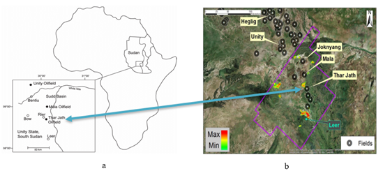
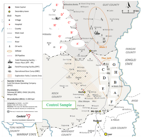
This research study was conduct in the Thar-Jath Oilfields of Unity State, South Sudan during dry and wet seasons as shown in Figure 1. Thar-Jath is a town found on the Unity Plateau in the eastern part of Unity State. The Thar-Jath plateau is located between latitude 8.743947°N and longitude 30.140401°E with an estimated area of 20,591 km2 forming the southernmost tip of the Unity State (Figure. 1a). The land-cover includes two main classes: black cotton soil (vertisol), a soil rich in montmorillonite (clay), and wetlands nearby the White Nile European Coalition on Oil in Sudan, (2003). With respect to the geological setting, the study area is inside the Muglad Basin that extends for 120,000 km2 from Sudan to South Sudan. The basin is composed of three rift cycles: Early Cretaceous (140–95 Ma), Late Cretaceous (95–65 Ma), Paleogene (65–30Ma) and well known for its hydrocarbon accumulations. The largest oilfields until now discovered are Heglig and Unity (Figure 1b): the first is outside Block 5A and the second adjoins the block. Inside Block 5A we find the Mala and Thar Jath oilfields that are well known for their Nile Blend, a medium low-sulfur waxy crude oil Pedersen et al., (2014).
Data Collection
Water Quality Index
The Water Quality Index (WQI) is widely used to assess and classify surface water quality. It is aggregate from many environmental parameters and expressed as a single value. In South Sudan, the WQI index is propose by the South Sudan Environment Administration to calculate the WQI index, at least 3 samples of parameters are required for the monitoring environment SSEA. (2019). In this study, 10 surface water quality parameters, including pH, temperature, DO, BOD, COD, NH4+-N, NO2– -N, NO3– -N, PO43--P, and coliform, were used to calculate the WQI index at zero monitoring locations during the dry and rainy seasons. The formula to calculate the WQI index is Equation 1:

Where: WQII is the WQI value of the pH parameter, WQIII is the WQI value for chemical variables (DO, BOD, COD, NH4+ -N, NO2– -N, NO3– -N and PO43- -P), and WQIIII is the WQI value for the biological variable (coliform). The scale of assessing surface water quality through the WQI index is divided into 6 levels, including (1) “Very heavily polluted” when WQI < 10, (2) “Poor” when WQI = 10-25, (3) “Bad” at WQI = 26-50, (4) “Medium” at WQI = 51-75, (5) “Good” at WQI = 76-90 and (6) “Very good” at WQI = 91-100. At the same time, the RBG color visually represents surface water quality at each monitoring location on the spatial map SSEA. (2019). WQI index map was produce using QGIS software version 3.28.
Risk Assessment
Environmental risks are often rapidly assessed using a risk quotient (RQ) and frequency of occurrence. RQ is calculate as the ratio between measured environmental concentrations (MECs) and concentrations predicted for no effect (PNEC), which is described as Equation 2 Xie et al., (2019). This study assessed the risks of 10 surface water pollution parameters, including TSS, BOD, COD, NH4+-N, NO2–-N, NO3–-N, PO43--P, Cl– , Fet and coliform.

In which PNEC was use as the limit value for surface water assessment. MEC is the concentration of pollutants measured at zero monitoring stations in the dry and rainy seasons. The RQ index rating scale is divided into four levels, including (1) if RQ is lower than 1, no risk is expected, (2) RQ ranges from 1 to 2, low impact is expected; RQ is between 2 and 3, moderate impact is expected and (3) RQ ≥ 3, the impact is high. Furthermore, the frequency of effects (F) was recorded base on the number of times it exceeds the limit value specified by Ministry of Water Resources. In which F > 70 % is assessed frequently, F range from 30 – 70% is moderate and F < 30% is infrequent. Finally, the risk classification of pollutants is carried out based on the matrix between RQ and F with 4 levels.
Pearson Correlation Analysis
Pearson correlation analysis was apply to find the relationship between WQI and RQ. When the correlation coefficient between variables close to 1 shows a strong positive correlation, the variable correlation coefficient close to -1 shows a robust negative correlation. Values close to 0 show no significant linear relationship. In this study, SPSS software version 20.0 was applied to Pearson correlation analysis for WQI and RQ values of all parameters used in calculating RQ at 8 sites in the dry and rainy seasons.
Principal Component Analysis
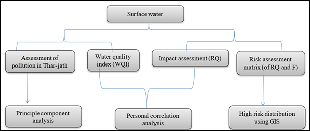
Principal component analysis (PCA) allows for the reduction of the original data set and forms new factors, mainly used to extract vital environmental variables and identify possible sources of surface water pollution. The Kaiser-Meyer-Olkin (KMO) and Bartlett tests were used to assess the fit of the PCA analysis dataset (Matta et al., 2020). In PCA analysis, the eigenvalue is often use to identify principal critical components (PCs). PCs with eigenvalues greater than 1 are retain to assess surface water quality variability. The loading factor between the environmental variables and the main component is divide into three levels: strong (>0.75), moderate (0.75-0.50), and weak (0.50- 0.30) Sharma et al., (2021). In this study, the purpose of the PCA analysis was to identify the main surface water variables affecting surface water quality during the dry and rainy seasons. This study used the average values of 12 surface water quality parameters at 8 monitoring stations in the dry and rainy seasons for PCA analysis using SPSS software version 20.0. The research methodology is present in a flowchart (Figure 3).
PAH s Risk Assessment
The environmental risk caused by PAHs was calculate considering the toxicity of individual PAHs. The toxicity equivalence factors (TEFs) of (USEPA 1993) were used for determining the toxicity. The TEFs and risk assessment standards (RASs) recommended in Cheng et al. (2011) were used in this study. Bap (TEF = 1, RAS = 0.1 mg/kg-1) was utilized as the reference chemical, and additional RASs were computed based on the ratio of Bap to the various PAHs. The ecological threat index was calculate by the mixture of the Nemerow index and ratio procedures using equation 3 below:
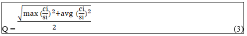
The Q value was use to divide the danger levels of PAHs in soil. Where Q stands for the environmental risk index, ci for individual PAH concentration in agricultural topsoil, si for individual PAH RAS value, and max and avg for the highest and average ci to si ratios, respectively. Specifically, “Q 1”, “1 < Q
3”, “3 < Q
6”, and “Q > 6” are the categories of safe, low risk, medium risk, and high risk.
Geo-Accumulation Index (Igeo)
This index is apply to quantify the metal pollution in the soils and aquatic sediments Rahman et al. (2022). It is calculated using equation 4:

Where Cn is the concentration of metal measured in sediment samples in the study area, Bn is the background value of the corresponding metal, and 1.5 is the background matrix correction due to lithological effects. According to Muller Rahman et al. (2022), the geo-accumulation index can be classified according to the following seven grades or classes as shown in the table 1.
| Classes | Ranges | Indication/water quality |
| 0 | Igeo<0 | Practically uncontaminated |
| 1 | 0 < Igeo<1 | Uncontaminated to moderately contaminated |
| 2 | 1 < Igeo<2 | Moderately contaminated |
| 3 | 2 < Igeo<3 | Moderately to heavily contaminated |
| 4 | 3 < Igeo<4 | Heavily contaminated |
| 5 | 4 < Igeo<5 | Heavily to extremely contaminated |
| 6 | 5< Igeo< | Extremely |
Table 1: Descriptive classes of Geo-accumulation index contamination factor risk factor.
Contamination Factor (CF)
The degree of contamination of each heavy metal element was also calculated using equation 5. The contamination factor was deem a useful tool to monitor contamination in soils over time (Ahamad et al. 2020). It is the ratio of every metal in the present sample to the background values in the same metal (Ahamad et al. 2020).
Enrichment Factor (EF)
EF for every metal is used to estimate how much metals originate from anthropogenic activities in the soils. The EF index was determined in the soil samples using equation 7 Luo et al., (2021):
Where Cn sample is the concentration of the heavy metal in the sample soil studied; Cn background is the concentrations in a suitable baseline reference material. Cn background is the average heavy metal concentration in the upper continental crust according to in mg/kg Mokhtarzadeh et al., (2020): Cr, 35; Cu, 14.3; Fe, 30890; Mn, Ni, 18.6; Pb, 17; Ni, 18.6; Hg, 0.056; CFe is the Fe content in the upper continental crust. So, the reference metal used to normalize the measured heavy metal concentration was Fe because of the low variation coefficient (CV) in all the soil samples Mokhtarzadeh et al. (2020). The significance of EF is as follows: EF < 1 indicates no enrichment, EF < 3 is minor enrichment, EF= 3–5 is moderate enrichment, EF= 5–10 is moderately severe enrichment, EF = 10–25 is severe enrichment, EF = 25–50 is very severe enrichment, and EF > 50 is extremely severe enrichment Luo et al. (2021).
Results & Discussions
Surface Water Quality Based on National Surface Water Quality Standards
The results in Table 2 show that only temperature, pH, and NO3 – -N in surface water in the study area were within the allowable limits of national technical regulations on surface water quality WHO (2013). Surface water in the study area was contaminate with suspended solids, organic matter, eutrophication, salinity, iron, and microbial contamination. pH, BOD, NH4+-N, PO43--P, and Fet in the water had statistically significant differences between the dry and rainy seasons (p<0.05). TSS fluctuated from 93.01±90.21 mg/L (dry season) to 92.97±68.30 mg/L (rainy season), an average of 4.64–4.65 times higher than the standard. This result is similar to the previous study by Rahman et al., (2022) in the surface water of Thar-jath province in 2024, exceeding 1.05–6.52 times. From that, it was conclude, that the TSS content in the water in 2024 tended to increase, higher than the previous year. However, high TSS was detect as lower than other coastal water bodies such as Warrap State and Lake State Khan et al., (2011). Meanwhile, TSS concentration tends to be higher than in areas with water bodies, (53.33±3.59- 59.59±8.82 mg/L) Hong et al. (2022). High-suspended solids in water are often associated with organic or inorganic contamination; moreover, they can also be carriers out by microbial contamination Wehrheim et al. (2023). DO in the surface water is very low, ranging from 2.79±0.33 mg/L during (dry season) to 2.72±0.37 mg/L during (rainy season). The low amount of oxygen in the water seriously affects the growth and development of aquatic species. The concentrations of the BOD, and COD for surface water range from 4.5±2.05-4.74±1.2 mg/L to 30.29±11.09-31.39±12.62 mg/L. The average seasonal variation of BOD and COD content has exceeded 1.1–1.2 times and 3.0–3.1 times compared with South Sudan standards, respectively. Lower BOD and COD concentrations were record compared to Warrap State and Lake State (Luo et al., 2023). In addition, the BOD content exceeded the regulatory limit insignificantly. Meanwhile, COD content is three times higher than the allowable limit in both rainy and dry seasons. This may be due to the fact that, Oilfields waste contains many substances that are difficult to biodegrade and industrial activities have increased COD content in surface water Cho et al. (2022). For the nutrients, NH4+-N fluctuated from 0.44±0.5 mg/L in the dry season to 0.58±0.56 mg/L in the rainy season, averaging about 1.5-1.9 times higher than the allowable limit. However, there is no significant difference between areas in Thar-Jath Luo et al. (2021). This is explained by the fact that NH4+-N concentrations are commonly highly concentrated in areas receiving large amounts of wastewater from aquaculture, domestic, industrial and rice cultivation. NO2– -N in the surface water bodies of State was 1.2 times higher than the allowable limit of QCVN 08-MT: 2015/BTNMT MoNRE. (2015). Compared with some other studies, the NO2–-N content in this study was relatively higher Unity State, namely Thar-Jath Jayasiri et al. (2022). This result is consistent with the measurement results of DO in water because the lack of oxygen in the water leads to incomplete nitrification. Consequently, the NO2–-N concentration in the water body increases Wehrheim et al., (2023). Moreover, high nitrite levels in water depend on agricultural fertilizer use and untreated wastewater discharge Drouiche et al. (2022). Organisms living in nitrite contaminated aquatic environments can experience oxidative stress in gills and serum, negatively affecting the growth and development of aquatic organisms Yang et al., (2020). On the other hand, PO43--P in surface water fluctuated from 0.12±0.42 mg/L (dry season) to 0.16±0.34 mg/L (rainy season), 1.2-1.6 times higher than the South Sudanese standard. NH4+-N and PO4 3--P were significantly higher in the rainy season than in the dry season (p to 0.16±0.34 mg/L (rainy season), 1.2-1.6 times higher than the South Sudanese standard. NH4+-N and PO43--P were significantly higher in the rainy season than in the dry season. The concentrations of Cl– the dry season and rainy seasons were record at 651.19±1291.33 mg/L and 286.11±498.83 mg/L, respectively. These results illustrated that Cl– was 21.87 times higher in the dry season compared to the QCVN 08-MT: 2015/BTNMT MoNRE. (2015). Meanwhile, the concentration of Cl in surface water in the rainy season was only 10 times higher than the standard. Fet concentration in the water exceeded the allowable limit of 4.5-5 times due to acid sulfate soil affecting water quality and the impact of untreated wastewater. Besides that, the previous study by Wehrheim et al. (2023) suggested that the increase of Fe in water is affect by aquaculture. Iron-rich water can cause odor, and taste problems and make the water corrosive Nguyen et al. (2020). The study results showed that coliform density fluctuated in the range of 18,158±20,639-24,497±49,896 MPN/100 mL, with an average of around 7-10 times higher than the standard. The activities of discharging wastewater from livestock, aquaculture and septic tanks of poor quality have seriously contaminated the water in this area with microorganisms. Coliform contamination in water bodies is widespread in Thar-Jath Hong et al. (2022).
| Serial No | Parameter | Unit | Dry season | Wet season | Min | Max | x QCSSD 08 MT:2021/BTNMT, A1 |
| 1 | Ph | – | 7.05±0.24a | 6.93±0.21b | 6.69 | 7.35 | 6-8.5 |
| 2 | Temp. | 30.24±1.07a | 30.43±1.27 | 29.27 | 31.70 | – | |
| 3 | TSS | mg/L | 93.01±90.21a | 92.97±68.30 | 23.73 | 240.17 | 20 |
| 4 | DO | mg/L | 2.79±0.33a | 2.72±0.37a | 2.22 | 3.49 | 6 |
| 5 | BOD | mg/L | 4.5±2.05b | 4.74±1.2a | 2.58 | 6.88 | 4 |
| 6 | COD | mg/L | 31.39±12.62a | 30.29±11.09a | 11.02 | 47.20 | 10 |
| 7 | NH4+ -N | mg/L | 0.44±0.5b | 0.58±0.56a | 0.03 | 2.21 | 0.3 |
| 8 | NO2—N | mg/L | 0.06±0.11a | 0.06±0.07a | 0.01 | 0.39 | 0.05 |
| 9 | NO3—N | mg/L | 0.27±0.2a | 0.26±0.14a | 0.10 | 0.54 | 2 |
| 10 | PO43—P | mg/L | 0.12±0.42b | 0.16±0.34a | 0.02 | 1.56 | 0.1 |
| 11 | Cl– | mg/L | 651.19±1291.33a | 286.11±498.83a | 18.86 | 3894.03 | 250 |
| 12 | Fet | mg/L | 2.32±1.79b | 2.62±1.55a | 0.81 | 5.37 | 0.5 |
| 13 | Coliform | MPN/100mL | 24,497±49,896a | 18,159±20,639a | 1,687 | 160,333 | 2500 |
Table 2: Summary of surface water quality.
Risk Assessment of Pollutants
The results of the impact level (RQ) and risk level ratio in the dry and rainy seasons are show in Table 3. TSS, COD, Fet and coliform parameters in the dry season were determined to have a high impact, with mean RQ values of 4.65, 3.14, 4.64 and 9.08, respectively. Furthermore, these parameters have medium and high-risk levels above 90% of the total sampling locations. Then there is Cl–, which was record with an RQ value of 2.60, assessed as having a moderate impact. However, the level of risk to the environment is only low (28.6%) and safe (37.1%) because the frequency of pollution in the dry season months is less than 30%. Next, BOD (RQ = 1.12), NH4+-N (RQ = 1.48), NO2–-N (RQ = 1.27) and PO43--P (RQ = 1.28) have environmental impacts and risks at low levels. Meanwhile, the impact and risks of NO3–-N on the water environment were not record.
Similarly, the level of impacts and risks in the rainy season tends to be similar to that in the dry season. TSS, COD, Fet and coliform were still recorded at high impact and the majority of sampling sites were at high risk. Nevertheless, the level of impact of Cl– on the environment in the rainy season is low, decreasing compared to the dry season. In contrast, the average RQ values of NH4+-N and PO43--P tended to increase the impact level but remained low. In addition, the environmental risk at the locations of these two parameters also increased, shifting from safe to low risk and low to moderate. In the dry season, only the E site was record with 7 out of 8 pollutants at high risk; this area is closest to the pipeline and the primary water source for aquaculture. Meanwhile, most of the locations with 3 – 5 out of 8 pollutants have a high risk; the sites are concentrated mainly in the Oil production areas. Therefore, if the type of Oilfields waste is not treat thoroughly before being discharge into the environment, it will bring many microorganisms and organic matter into the receiving environment. Organic matter and microorganisms will consume large amounts of oxygen in the water, reducing oxygen levels and disrupting aquatic life Hamed et al. (2019). In the rainy season, the distribution of locations with a number of high-risk parameters was similar to that of the dry season. However, the number of sites with pollutants at a high environmental risk tended to increase more than in the dry season. Specifically, there are 5 out of 8 positions with many parameters at high-risk level, with about 5-6 parameters.
| Par. | Dry season | Rainy season | ||||||||||||
| RQ | Risk level ratio (%) | RQI | Risk level ratio (%) | |||||||||||
| Mean | Min | Max | N | L | M | H | Mean | Min | Max | N’ | L’ | M’ | H’ | |
| TSS | 4.65 | 1.19 | 12.01 | 0.0 | 5.7 | 40.0 | 54.3 | 4.65 | 1.92 | 8.76 | 0.0 | 2.9 | 34.3 | 62.9 |
| BOD | 1.12 | 0.65 | 1.72 | 8.6 | 85.7 | 5.7 | 0.0 | 1.18 | 0.73 | 1.57 | 8.6 | 88.6 | 2.9 | 0.0 |
| COD | 3.14 | 1.42 | 4.72 | 0.0 | 8.6 | 34.3 | 57.1 | 3.03 | 1.10 | 4.21 | 0.0 | 1.71 | 22.9 | 60.0 |
| NH₄⁺-N | 1.48 | 0.11 | 6.04 | 25.7 | 45.7 | 17.1 | 11.4 | 1.94 | 0.12 | 7.38 | 20.0 | 31.4 | 31.4 | 17.1 |
| NO₂ˉ-N | 1.27 | 0.12 | 7,57 | 43.3 | 54.4 | 11.4 | 2.9 | 1.19 | 0.16 | 3.80 | 42.9 | 34.3 | 20.0 | 2.9 |
| NO₃ˉ-N | 0.14 | 0.05 | 0.26 | 100 | 0.0 | 0.0 | 0.0 | 0.13 | 0.05 | 0.27 | 100 | 0.0 | 0.0 | 0.0 |
| PO₄³ˉ-P | 1.28 | 0.22 | 15.56 | 54.3 | 34.3 | 8.6 | 2.9 | 1.56 | 0.21 | 12.89 | 34.3 | 54.3 | 2.9 | 8.6 |
| Clˉ | 2.60 | 0.12 | 15.58 | 37.1 | 28.6 | 14.3 | 20.0 | 1.14 | 0.08 | 6.60 | 60.0 | 20.0 | 5.7 | 14.3 |
| Fet | 4.64 | 1.62 | 10.75 | 0.0 | 5.7 | 22.9 | 71.4 | 5.24 | 1.87 | 9.71 | 0.0 | 2.9 | 11.4 | 85.7 |
| coliform | 9.80 | 0.67 | 64.13 | 0.0 | 11.4 | 31.4 | 57.1 | 7.26 | 1.27 | 24.0 | 0.0 | 11.4 | 42.9 | 45.7 |
| Note: ** Correlation is significant at the 0.01 level (2-tailed) | ||||||||||||||
Table 3: Seasonal changes of RQ and risk level ratio of water pollutants.
Correlation between Overall Surface Water Quality and Risk Quotient
The correlation between the water quality index (WQI) and the impact level of pollutants (R-Qi) are present in Table 4. During the dry season, the WQI was negatively correlated with RQ-BOD, RQ-COD, RQ-NH₄⁺-N and RQ-coliform, with the correlation coefficients of (-0.611), (-0.499), (-0.493) and (-0.445), respectively. During the rainy season, the WQI index had a significant negative correlation with RQ-BOD (r = -0.703), RQ-COD (r = -0.559), RQ-NH₄⁺-N (r = -0.531), RQ-Fet (r = -0.512) and RQ-coliform (r = -0.653) at 1% significance level. Moreover, WQI showed a significant positive correlation with RQNO₃ˉ-N (r = 0.471), indicating that NO3–-N does not affect the environment. The results of correlation analysis show that the lower the WQI index, the higher the impact level and vice versa. In the dry season, WQI index values range from 26-91, dividing surface water quality into four quality levels: very good, good, medium and bad. Only one site (control) has very good water quality, accounting for 2.86% of the total samples. Good water quality was determined at 3 locations, including L, M, and H (accounting for 14.29% of the total samples). The medium water quality accounted for 22.86% of the total samples found at locations L, and M. Bad water quality accounted for 60% of total samples, including positions R, and P. During the rainy season, WQI values fluctuated between 31 and 88, classifying surface water quality into three levels good, medium and bad. Sites with good water quality accounted for 17.14% of the total sample, including site M. Locations with medium water quality accounted for 20% of the total samples, including M, and H. About 63% of the total samples (4 locations) had bad water quality during the rainy season compared with the study of Luo et al. (2021), the WQI in Unity shows that water quality is heavily polluted and poor.
| Index | WQI_Dry season | WQI_Rainy season | ||
| R | P | R | P | |
| RQ-TSS | 0.088 | 0.615 | -0.182 | 0.297 |
| RQ-BOD | -0.611** | 0.000 | -0.703** | 0.000 |
| RQ-COD | -0.499** | 0.002 | -0.559** | 0.000 |
| RQ-NH₄⁺-N | -0.493** | 0.003 | -0.531** | 0.001 |
| RQ-NO₂ˉ-N | -0.324 | 0.058 | -0.300 | 0.080 |
| RQ-NO₃ˉ-N | 0.199 | 0.253 | 0.471** | 0.004 |
| RQ-PO₄³ˉ-P | -0.271 | 0.115 | -0.065 | 0.709 |
| RQ-Clˉ | 0.142 | 0.415 | -0.058 | 0.739 |
| RQ-Fet | -0.067 | 0.702 | -0.512** | 0.002 |
| RQ-coliform | -0.445** | 0.007 | -0.653** | 0.000 |
| Note: ** Correlation is significant at the 0.01 level (2-tailed) | ||||
Table 4: Correlation between overall surface water quality and risk quotient
| Water | |||||||
| As | Ca | Cd | Cu | Fe | Pb | Zn | |
| As | 1 | ||||||
| Ca | 0.798 | 1 | |||||
| Cd | 0.441 | 0.746 | 1 | ||||
| Cu | -0.219 | -0.181 | 0.005 | 1 | |||
| Fe | -0.041 | -0.149 | -0.162 | 0.051 | 1 | ||
| Pb | -0.264 | -0.282 | -0.116 | 0.135 | 0.900 | 1 | |
| Zn | 0.395 | 0.724 | 0.984 | 0.0001 | -0.701 | -0.011 | 1 |
Table 5: Correlation coefficients of heavy metal concentrations in surface water.
| Cu | Pb | Zn | As | Cd | Ba | |
| Cu | 1 | |||||
| Pb | 0.644(*) | 1 | ||||
| Zn | 0.356 | 0.178 | 1 | |||
| As | 0.291 | 0.402 | 0.708(**) | 1 | ||
| Cd | 0.498 | 0.646(*) | 0.726(**) | 0.613(*) | 1 | |
| Ba | 0.605 (*) | 0.673(*) | 0.387 | 0.476 | 0.558(*) | 1 |
| Notes: N/A means not available. | ||||||
Table 6: Correlation coefficient of trace elements for stream sediment.
Bold indicates TDS value above the permissible limit.
* Correlation is significant at the 0.05 level (2-tailed).
** Correlation is significant at the 0.01 level (2-tailed).
The correlation matrix in water showed very strong and positive correlation. Geochemical environment are essential elements necessary for the growth of both plants and animals in the study area (Table 3.6). correlation coefficient for trace metals for stream sediment showed that Pb–Cu, Ba–Cu, Cd–Pb, As–Zn, Cd–Zn, Ba–Cd with ‘r’ values 0.644, 0.673, 0.646, 0.708, 0.726, 0.558 are all influenced from the same anthropogenic source in the study area as shown in Table 5. The correlation coefficients between PAHs, granularity, pH, and TOC (%) are given in Table 7. From the results, the findings showed that there was a negative correlation of PAHs with pH except for AC, Fluo, and AN. The PAHs show a positive relationship with the percentage of TOC (%), except AC, Fluo, and AN, which may be due to a positive correlation between the pH and polarization of the soil organic matter, which decreases PAHs adsorption into soil organic matter by an increase in pH. Zhou et al. (2019) outlined that the TOC is a critical factor in describing the transportation of PAHs in top soils. The 8 PAHs show a significant positive correlation with TOC (%), except AC, Fluo, and AN.
| PAHs | NA | AC | ACY | Fluo | Phen | AN | Flur | Pye | Ph | TOC |
| NA | 1 | |||||||||
| AC | 0.61 | 1 | ||||||||
| ACY | 0.71 | 0.55 | 1 | |||||||
| Fluo | 0.47 | 0.47 | 0.34 | 1 | ||||||
| Phen | 0.45 | 0.48 | 0.54 | 0.31 | 1 | |||||
| AN | 0.41 | 0.61 | 0.36 | 0.53 | 0.28 | 1 | ||||
| Flur | 0.38 | 0.45 | 0.23 | 0.42 | 0.57 | 0.48 | 1 | |||
| Pye | 0.30 | 0.30 | 0.29 | 0.41 | 0.27 | 0.41 | 0.53 | 1 | ||
| pH | −0.44 | 0.15 | −0.17 | 0.28 | −0.12 | 0.18 | −0.11 | −0.17 | 1 | |
| TOC | 0.08 | 0.03 | 0.22 | 0.05 | 0.38 | 0.29 | 0.26 | 0.28 | 0.18 | 1 |
Table 7: related coefficients between PAHs and pH, TOC, and granularity of agricultural top soils.
However, this is due to PAHs’ hydrophobic nature, which combines with the soil organic matter after PAHs enter the soil. Moreover, the PAHs show a negative correlation with clay and slit, whereas a positive correlation with sand.
| PAHs | Environmental Risks Index (Q) | Q | 1 | 3 | Q |
| NA | 2.76 | – | 1 | – | – |
| AC | 1.91 | – | 1 | – | – |
| ACY | 3.87 | – | – | 1 | – |
| Fluo | 2.91 | – | 1 | – | – |
| Phen | 3.78 | – | – | 1 | – |
| AN | 6.61 | – | – | – | 1 |
| Flur | 4.95 | – | – | 1 | – |
| Pye | 4.87 | – | – | 1 | – |
Table 8: The environmental risk index values for the individual PAHs in agricultural top soils.
The environmental risk assessment shows that the Thar-jath areas were at low to high risk. The ecological risk index values in Table 8, indicates that the PAHs NA, AC, and Fluo cause low risk, whereas the PAHs ACY, Phen, Flur, and Pye cause medium risk. The high molecular weight (HMW) PAHs cause high risk in the Thar-jath agricultural topsoil sampling areas. Thus, this Thar-jath area poses a high environmental risk due to PAH pollution in agricultural topsoil.
Contamination Factor (CF), Enrichment Factor (EF) evaluation of the metals
Contamination Factor (CF), Site B, and C at 0-10cm, and 10-60cm B & C show low to moderate contamination for all the studied heavy metals (Table 10), while site A shows low pollution for Cr (A) and Ni (A & at 10-30cm A). Site A at 0-10cm & 10-30cm site A) showed moderate pollution for Cd, Pb, Hg, and Mn but showed very high pollution for Cu (A), considerable pollution for Cu at 10-30cm (A), and considerable pollution for Fe (A at 0-10cm & 10-30cm A). Site B and C which are soils from agricultural farms show low to moderate pollution indicating probably less use of agro-chemicals. EF was use to estimate how much metals originated from anthropogenic activities in the soils. For Pb, Fe, Ni, and Mn, there is no enrichment for all the sites but for Cr, there is moderate enrichment for the control and A (topsoil) but no enrichment for the other sites. This indicates that the principal source of these metals was mainly from crust material. Though the concentration of Cd ranged from 1.75 to 6.49 mg/kg in all the sites, EF values were very high for all the sites indicating very severe enrichment for the control, A, and at (10-30cm), severe enrichment for B and C and extremely severe enrichment for A as shown in. Hg at (10-30cm), had extremely severe enrichment status for all the sites while at (0-10cm), Cu had severe enrichment for sites B, C, at (10-30cm) C; moderately severe enrichment for the control, minor enrichment for A at (0-10cm) and very severe enrichment for A at (10-30cm). In almost all the cases where there was enrichment (Cd, Cr, Cu, Hg), the values of subsurface samples were higher than those for surface samples (Table 11). These shows the high mobility of these heavy metals in these soils as they are mainly sandy soil and they could be transported into adjacent soils as well as contaminate the underground water. The high EF values are due to contributions of anthropogenic sources mainly agricultural activities and the use of chemicals in the post-treatment of the sites with petroleum activities.
| Cr | Cd | |||||||
| site | Igeo | Class interval | Significance | Igeo | Class interval | Significance | ||
| A (0-10cm) | -0.671 | Igeo ≤ 0 | No pollution | -0.325 | Igeo ≤ 0 | No pollution | ||
| A (10-30cm) | -0.408 | Igeo ≤ 0 | No pollution | 0.295 | Igeo = 0-1 | No to moderate pollution | ||
| B(0-10cm) | -3.689 | Igeo ≤ 0 | No pollution | -0.088 | Igeo ≤ 0 | No pollution | ||
| B(10-30cm) | -3.661 | Igeo ≤ 0 | No pollution | -1.545 | Igeo ≤ 0 | No pollution | ||
| C(0-10cm) | -4.304 | Igeo ≤ 0 | No pollution | -1.605 | Igeo ≤ 0 | No pollution | ||
| C(10-30cm) | -5.263 | Igeo ≤ 0 | No pollution | -0.181 | Igeo ≤ 0 | No pollution | ||
| D (0-10cm) | -0.686 | Igeo ≤ 0 | No pollution | -0.325 | Igeo ≤ 0 | No pollution | ||
| D (10-30cm) | -0.298 | Igeo ≤ 0 | No pollution | 0.289 | Igeo = 0-1 | No to moderate pollution | ||
| Pb | Hg | |||||||
| site | Igeo | Class interval | Significance | Igeo | Class interval | Significance | ||
| A (0-10cm) | 4.212 | Igeo | Highly polluted | 0.121 | Igeo = 0-1 | No to moderate pollution | ||
| A (10-30cm) | 2.092 | Igeo | moderate pollution | 0.136 | Igeo = 0-1 | No to moderate pollution | ||
| B(0-10cm) | 2.1 | Igeo | No to moderate pollution | -2.532 | Igeo ≤ 0 | No pollution | ||
| B(10-30cm) | 1.212 | Igeo | moderate pollution | -3.064 | Igeo ≤ 0 | No pollution | ||
| C(0-10cm) | 1.595 | Igeo | moderate pollution | -3.640 | Igeo ≤ 0 | No pollution | ||
| C(10-30cm) | 0.170 | Igeo ≤ 0 | No pollution | -3.863 | Igeo ≤ 0 | No pollution | ||
| D (0-10cm) | 0.212 | Igeo =0-1 | No to moderate pollution | 0.121 | Igeo = 0-1 | No to moderate pollution | ||
| D (10-30cm) | -0.092 | Igeo ≤ 0 | No pollution | 0.136 | Igeo = 0-1 | No to moderate pollution | ||
| Cu | Zn | |||||||
| site | Igeo | Class interval | Significance | Igeo | Class interval | Significance | ||
| A (0-10cm) | 2.246 | Igeo =2-3 | Moderate to heavy pollution | 0.479 | Igeo ≤ 0 | No to moderate pollution | ||
| A (10-30cm) | 1.615 | Igeo =1-2 | moderate pollution | 0.451 | Igeo ≤ 0 | No to moderate pollution | ||
| B(0-10cm) | 0.351 | Igeo =0-1 | No to moderate pollution | -4.510 | Igeo ≤ 0 | No pollution | ||
| B(10-30cm) | 1.212 | Igeo | moderate pollution | -3.064 | Igeo ≤ 0 | No pollution | ||
| C(0-10cm) | 1.595 | Igeo | moderate pollution | -3.640 | Igeo ≤ 0 | No pollution | ||
| C(10-30cm) | 0.170 | Igeo ≤ 0 | No pollution | -3.863 | Igeo ≤ 0 | No pollution | ||
| D (0-10cm) | 2.256 | Igeo =2-3 | Moderate to heavy pollution | 0.489 | Igeo ≤ 0 | No to moderate pollution | ||
| D (10-30cm) | 1.615 | Igeo =1-2 | moderate pollution | 0.446 | Igeo ≤ 0 | No to moderate pollution | ||
| Fe | Ni | |||||||
| site | Igeo | Class interval | Significance | Igeo | Class interval | Significance | ||
| A (0-10cm) | 1.276 | Igeo =1-2 | Moderate pollution | -0.942 | Igeo ≤ 0 | No pollution | ||
| A (10-30cm) | 1.101 | Igeo =1-2 | Moderate pollution | -0.912 | Igeo ≤ 0 | No pollution | ||
| B(0-10cm) | 2.685 | Igeo ≤ 0 | Moderate pollution | -0.832 | Igeo ≤ 0 | No pollution | ||
| B(10-30cm) | 1.827 | Igeo ≤ 0 | Moderate pollution | -0.712 | Igeo ≤ 0 | No pollution | ||
| C (0-10cm) | 3.748 | Igeo ≤ 0 | Highly polluted | -0.937 | Igeo ≤ 0_ _ | No pollution | ||
| C (10-30cm) | 2.192 | Igeo ≤ 0 | moderate pollution | -1.237 | Igeo ≤ 0_ _ | No pollution | ||
| D (0-10cm) | 0.212 | Igeo =0-1 | No to moderate pollution | 0.121 | Igeo = 0-1 | No to moderate pollution | ||
| D (10-30cm) | -0.092 | Igeo ≤ 0 | No pollution | 0.136 | Igeo = 0-1 | No to moderate pollution | ||
Table 9: Variation of Igeo values and significance for each heavy metal in soil at different study sites.
| Cr | Cd | |||||
| site | CF | Class interval | Significance | CF | Class interval | Significance |
| A (0-10cm) | 0.945 | CF ˂ 1 | low pollution | 1.212 | 1 ˂ CF ˂ 3 | moderate pollution |
| A (10-30cm) | 1.168 | 1 ˂ CF ˂ 3 | moderate pollution | 1.848 | 1 ˂ CF ˂ 3 | moderate pollution |
| B(0-10cm) | 0.125 | CF ˂ 1 | low pollution | 1.416 | 1 ˂ CF ˂ 3 | moderate pollution |
| B(10-30cm) | 0.128 | CF ˂ 1 | low pollution | 0.512 | CF ˂ 1 | low pollution |
| C(0-10cm) | 0.078 | CF˂ 1 | low pollution | 0.513 | CF ˂ 1 | low pollution |
| C(10-30cm) | 0.049 | CF ˂ 1 | low pollution | 1.342 | 1˂ CF ˂ 3 | moderate pollution |
| D (0-10cm) | 0.945 | CF ˂ 1 | low pollution | 1.216 | 1 ˂ CF ˂ 3 | moderate pollution |
| D (10-30cm) | 1.238 | 1 ˂ CF ˂ 3 | moderate pollution | 1.848 | 1 ˂ CF ˂ 3 | moderate pollution |
| Pb | Hg | |||||
| A (0-10cm) | 7.165 | CF ˃ 6 | very high pollution | 2.14 | 1 ˂ CF ˂ 3 | moderate pollution |
| A (10-30cm) | 4.558 | 3 ˂ CF ˂ 6 | considerable pollution | 2.0372 | 1 ˂ CF ˂ 3 | moderate pollution |
| B(0-10cm) | 1.923 | 1 ˂ CF ˂ 3 | moderate pollution | 0.061 | CF ˂ 1 | low pollution |
| B(10-30cm) | 2.534 | 1 ˂ CF ˂ 3 | moderate pollution | 0.631 | CF ˂ 1 | low pollution |
| C(0-10cm) | 1.665 | 1 ˂ CF ˂ 3 | moderate pollution | 0.094 | CF ˂ 1 | low pollution |
| C(10-30cm) | 2.985 | 1 ˂ CF ˂ 3 | moderate pollution | 0.148 | CF ˂ 1 | low pollution |
| D (0-10cm) | 7.062 | CF ˃ 6 | very high pollution | 2.13 | 1 ˂ CF ˂ 3 | moderate pollution |
| D (10-30cm) | 4.663 | 3 ˂ CF ˂ 6 | considerable pollution | 2.137 | 1 ˂ CF ˂ 3 | moderate pollution |
| Cu | Zn | |||||
| A (0-10cm) | 1.753 | 1 ˂ CF ˂ 3 | moderate pollution | 1.626 | 1 ˂ CF˂ 3 | moderate pollution |
| A (10-30cm) | 1.412 | 1 ˂ CF ˂ 3 | moderate pollution | 1.642 | 1 ˂ CF ˂ 3 | moderate pollution |
| B(0-10cm) | 2.75 | 1 ˂ CF ˂ 3 | moderate pollution | 0.251 | CF ˂ 1 | low pollution |
| B(10-30cm) | 1.75 | 1 ˂ CF ˂ 3 | moderate pollution | 0.129 | CF ˂ 1 | low pollution |
| C(0-10cm) | 1.23 | 1 ˂ CF ˂ 3 | moderate pollution | 0.126 | CF ˂ 1 | low pollution |
| C(10-30cm) | 0.627 | CF ˂ 1 | low pollution | 0.114 | CF ˂ 1 | low pollution |
| D (0-10cm) | 1.782 | 1 ˂ CF ˂ 3 | moderate pollution | 1.626 | 1 ˂ CF˂ 3 | moderate pollution |
| D (10-30cm) | 1.412 | 1 ˂ CF ˂ 3 | moderate pollution | 1.647 | 1 ˂ CF ˂ 3 | moderate pollution |
| Fe | Ni | |||||
| A (0-10cm) | 3.618 | 3 ˂ CF ˂ 6 | considerable pollution | 0.791 | CF ˂ 1 | low pollution |
| A (10-30cm) | 3.216 | 3 ˂ CF ˂ 6 | considerable pollution | 0.864 | CF ˂ 1 | low pollution |
| B(0-10cm) | 0.949 | CF ˂ 1 | low pollution | 0.789 | CF ˂ 1 | low pollution |
| B(10-30cm) | 0.916 | CF ˂ 1 | low pollution | 0.927 | CF ˂ 1 | low pollution |
| C(0-10cm) | 0.548 | CF ˂ 1 | low pollution | 0.796 | CF ˂ 1 | low pollution |
| C(10-30cm) | 0.664 | CF ˂ 1 | low pollution | 0.646 | CF ˂ 1 | low pollution |
| D (0-10cm) | 3.618 | 3 ˂ CF ˂ 6 | considerable pollution | 0.886 | CF ˂ 1 | low pollution |
| D (10-30cm) | 3.216 | 3 ˂ CF ˂ 6 | considerable pollution | 0.859 | CF ˂ 1 | low pollution |
Table 10: Variation of CF values and significance for each heavy metal in soil at different study sites
| Cr | Cd | |||||
| site | EF | Interval | significance | EF | Interval | significance |
| Control | 4.979 | 3˂EF˂5 | moderate enrichment | 34.814 | 25˂EF˂50 | very severe enrichment |
| A (0-10cm) | 4.697 | 3˂EF˂5 | moderate enrichment | 41.971 | 25˂EF˂50 | very severe enrichment |
| A (10-30cm) | 5.687 | EF˂1 | no enrichment | 63.677 | EF > 50 | extremely severe enrichment |
| B(0-10cm) | 0.579 | EF˂1 | no enrichment | 49.168 | 25˂EF˂50 | very severe enrichment |
| B(10-30cm) | 0.589 | EF˂1 | no enrichment | 17.697 | 10˂EF˂25 | severe enrichment |
| C (0-10cm) | 4.697 | 3˂EF˂5 | moderate enrichment | 42.971 | 25˂EF˂50 | very severe enrichment |
| C (10-30cm) | 5.687 | EF˂1 | no enrichment | 62.677 | EF > 50 | extremely severe enrichment |
| D (0-10cm) | 0.579 | EF˂1 | no enrichment | 46.168 | 25˂EF˂50 | very severe enrichment |
| D (10-30cm) | 0.589 | EF˂1 | no enrichment | 19.697 | 10˂EF˂25 | severe enrichment |
| Pb | Hg | |||||
| Site | EF | Interval | significance | EF | Interval | significance |
| Control | 0.0017 | EF˂1 | no enrichment | 5799.117 | EF > 50 | extremely severe enrichment |
| A (0-10cm) | 0.0014 | EF˂1 | no enrichment | 9395.214 | EF > 50 | extremely severe enrichment |
| A (10-30cm) | 0.0012 | EF˂1 | no enrichment | 9491.357 | EF > 50 | extremely severe enrichment |
| B (0-10cm) | 0.0014 | EF˂1 | no enrichment | 1514.164 | EF > 50 | extremely severe enrichment |
| B (10-30cm) | 0.0012 | EF˂1 | no enrichment | 1038.786 | EF > 50 | extremely severe enrichment |
| C (0-10cm) | 4.697 | 3˂EF˂5 | moderate enrichment | 45.971 | 25˂EF˂50 | very severe enrichment |
| C (10-30cm) | 5.687 | EF˂1 | no enrichment | 53.677 | EF > 50 | extremely severe enrichment |
| D (0-10cm) | 0.579 | EF˂1 | no enrichment | 48.168 | 25˂EF˂50 | very severe enrichment |
| D (10-30cm) | 0.589 | EF˂1 | no enrichment | 18.697 | 10˂EF˂25 | severe enrichment |
| Cu | Zn | |||||
| Site | EF | Interval | significance | EF | Interval | significance |
| Control | 8.062 | 5˂EF˂10 | moderately enrich | 0.161 | EF˂1 | no enrichment |
| A (0-10cm) | 7.110 | EF > 50 | minor enrichment | 0.326 | EF˂1 | no enrichment |
| A (10-30cm) | 36.828 | 25˂EF˂50 | severe enrichment | 0.318 | EF˂1 | no enrichment |
| B (0-10cm) | 15.438 | 10˂EF˂25 | severe enrichment | 0.011 | EF˂1 | no enrichment |
| B (10-30cm) | 20.496 | 10˂EF˂25 | severe enrichment | 0.096 | EF˂1 | no enrichment |
| C (0-10cm) | 4.697 | 3˂EF˂5 | moderate enrichment | 41.971 | 25˂EF˂50 | very severe enrichment |
| C (10-30cm) | 5.687 | EF˂1 | no enrichment | 67.677 | EF > 50 | extremely severe enrichment |
| D (0-10cm) | 0.579 | EF˂1 | no enrichment | 46.168 | 25˂EF˂50 | very severe enrichment |
| D (10-30cm) | 0.589 | EF˂1 | no enrichment | 16.697 | 10˂EF˂25 | severe enrichment |
| Fe | Ni | |||||
| Site | EF | Interval | significance | EF | Interval | significance |
| Control | 0.0008 | EF˂1_ _ | no enrichment | 0.008 | EF˂1 | no enrichment |
| A (0-10cm) | 0.0014 | EF˂1 | no enrichment | 0.003 | EF˂1 | no enrichment |
| A (10-30cm) | 0.0013 | EF˂1 | no enrichment | 0.004 | EF˂1 | no enrichment |
| B (0-10cm) | 0.0015 | EF_˂1 | no enrichment | 0.004 | EF˂1 | no enrichment |
| B(01-30cm) | 0.0015 | EF˂1 | no enrichment | 0.005 | EF˂1 | no enrichment |
| C (0-10cm) | 4.697 | 3˂EF˂5 | moderate enrichment | 41.971 | 25˂EF˂50 | very severe enrichment |
| C (10-30cm) | 5.687 | EF˂1 | no enrichment | 63.677 | EF > 50 | extremely severe enrichment |
| D (0-10cm) | 0.579 | EF˂1 | no enrichment | 49.168 | 25˂EF˂50 | very severe enrichment |
| D (10-30cm) | 0.589 | EF˂1 | no enrichment | 17.697 | 10˂EF˂25 | severe enrichment |
Table 11: Variation of EF values and significance for each heavy metal at different study sites.
EF was use to estimate how much metals originated from anthropogenic activities in the soils. For Pb, Fe, Ni, and Mn, there is no enrichment for all the sites but for Cr, there is moderate enrichment for the control and A (topsoil) but no enrichment for the other sites (Table 11). This indicates that the principal source of these metals was mainly from crust material. Though the concentration of Cd ranged from 1.75 to 6.49 mg/kg in all the sites, EF values were very high for all the sites indicating very severe enrichment for the control, A, and at (10-30cm), severe enrichment for B and C and extremely severe enrichment for A as shown in (Table 11).
Conclusion
Surface water quality in the study area have been contaminate with organic matter, nutrients, microorganisms, salinity, and iron. The WQI index in the dry season was assess from bad to very good and from bad to good in the rainy season. The impact level of TSS, COD, Fet, and coliform in both seasons was recorded at a high impact and the risk level of these parameters in the centralized environment is medium and high. The distribution of high-risk pollutants is concentrated in residential and coastal areas. The negative correlation between the WQI index and the RQ index of BOD, COD, NH4+-N, Fet, and coliform indicated low overall water quality as the impact was high. The water quality indicators that pose ecological risks in the studied water bodies include TSS, BOD, COD, NH4+-N, PO43--P, Cl–, Fet, and coliform derived from natural conditions (acid sulfate soil, rainwater runoff), wastewater (domestic, aquaculture, livestock, cultivation, industry), and seawater intrusion. The results show that further strengthening management system is require for monitoring the quality of surface water to minimize environmental risks. In order to control this pollution, it can be minimized or remediated with water hyacinth introduced as the possible interaction between the modified plant and contaminated soil. FTIR, SEM, and XRD techniques can be employed to investigate soil and fresh water hyacinth plant and dried water hyacinth plant roots in post-remediation processes in a selected oilfield in South Sudan with the aim to evaluate the efficacy of remediation.
Acknowledgements
The support for this research was made possible through a capacity building competitive grant training the next generation of scientists provided by the Carnegie Cooperation of New York through the Regional Universities Forum for Capacity Building in Agriculture (RUFORUM). GTA Grant; Grant# RU/2024/GTA/CCNY/05).
Author Contributions
Prof.FOZAO KENNEDY FOLEPAI, Prof. TSAMO CORNELIUS facilitated and conceptualized the whole research process and write-ups construction; Prof. CHEO EMMANUEL SUH edited and proofread the final paper; BIOR J. AKOI conducted the research, analyzed the data, and wrote the paper; all authors approved the final revision of the paper.
Declarations
Conflict of interest on behalf of all authors; the corresponding author states that there is no conflict of interest.
References
- Andretta M, Coppola F, Modelli A, Santopuoli N, Seccia L. Proposal for a new environmental risk assessment methodology in cultural heritage protection. Journal of Cultural Heritage. 2017; 23:22-32.
- Ahamad, M. I, Song, J, Sun, H, Wang, X, Mehmood, M. S, Sajid, M, Su, P. and. Khan, A. J. (2020). Contamination Level, Ecological Risk, and Source Identification of Heavy Metals in the Hyporheic Zone of the Weihe River, China. Int. J. Environ. Res. Public Health, 17:1070
- An, Y. Study on Risk Assessment and Early Warning of Groundwater Pollution in the Ordos Basin. Master’s Thesis, Jilin University, Changchun, China, 2016.
- Bare JC. TRACI: The tool for the reduction and assessment of chemical and other environmental impacts. Journal of industrial ecology. 2002; 6(3-4):49-78.
- Blivband Z, Grabov P, Nakar O, editors. Expanded FMEA (EFMEA). Annual Symposium Reliability and Maintainability, 2004 – RAMS; 2004 26-29 Jan. 2004.
- Chang, K. The Effect of Iron Catalyst on Oxidation of Oil Contaminated Soil. Master’s Thesis, Xi’an University of Architecture and Technology, Xi’an, China, 2013.
- Enick OV, Moore MM. Assessing the assessments: pharmaceuticals in the environment. Environmental Impact Assessment Review. 2007; 27(8):707-29.
- Hakanson, L., (1980). An ecological risk index for aquatic pollution control a sedimentological approach. Water Res. 14, 975–1001.
- Hamed, M. A. R. (2019). Application of Surface Water Quality Classification Models Using Principal Components Analysis and Cluster Analysis. SSRN Electronic Journal.
- Hong, T., Viet, L., & Giao, N. (2022). Analysis of Spatial-Temporal Variations of Surface Water Quality in the Southern Province of Vietnamese Mekong Delta Using Multivariate Statistical Analysis. Journal of Ecological Engineering, 23(7), 1–9.
- Jalali I, Poorhashemi SM, Mirjalili A. Investigating Environmental Impact Assessment (EIA) In Early Studies (Zero-Phase) to Prevent Delay in Operation of Construction Projects. Civil Engineering Journal. 2018;4(1):117-25.
- Jayasiri, M. M. J. G. C. N., Yadav, S., Dayawansa, N. D. K., Propper, C. R., Kumar, V., & Singleton, G. R. (2022). Spatio-temporal analysis of water quality for pesticides and other agricultural pollutants in Deduru Oya river basin of Sri Lanka. Journal of Cleaner Production, 330, 129897.
- Jozi SA, Seyfosadat SH. Environmental risk assessment of Gotvand-Olia dam at operational phase using the integrated method of environmental failure mode and effects analysis (EFMEA) and preliminary hazard analysis. Journal of Environmental Studies. 2014; 4 0(1):25.
- Kaliraj, S.; Chandrasekar, N.; Peter, T.S.; Selvakumar, S.; Magesh, N.S. Mapping of coastal aquifer vulnerable zone in the south west coast of Kanyakumari, South India, using GIS-based DRASTIC model. Environ. Monit. Assess. 2015, 187, 4073.
- Khan, M. A., & Ghouri, A. M. (2011). Environmental pollution: its effects on life and its remedies. Researcher World: Journal of Arts, Science & Commerce, 2(2), 276-285.
- Khan, R.; Jhariya, D.C. Assessment of Groundwater Pollution Vulnerability Using GIS Based Modified DRASTIC Model in Raipur City, Chhattisgarh. J. Geol. Soc. India 2019, 93, 293–304.
- Luo, Y. and Jia, Q. (2021). Pollution and Risk Assessment of Heavy Metals in the Sediments and Soils around Tiegelongnan Copper Deposit, Northern Tibet, China. Journal of Chemistry Volume, Article,
- Makvandi R, Astani S, Cheraghi M. Environmental risk assessment of wetlands using SAW and EFMEA (Case study: international wetland Anzali). Wetland Ecobiology. 2013; 5(3):61-72.
- Medici, G.; Engdahl, N.B.; Langman, J.B. A Basin-Scale Groundwater Flow Model of the Columbia Plateau Regional Aquifer System in the Palouse (USA): Insights for Aquifer Vulnerability Assessment. Int. J. Environ. Res. 2021, 15, 299–312.
- Miao, Y. The way, harm and preventive measures of groundwater pollution caused by oil exploitation. Water Resour. Dev. Res. 2016, 5, 32–33.
- Misra V, Pandey SD. Hazardous waste, impact on health and environment for development of better waste management strategies in future in India. Environment International. 2005; 31(3):417-31.
- Mokhtarzadeh, Z, Keshavarzi, B, Moore, F, Marsan, F.A. and Padoan, E. (2020). Potentially toxic elements in the Middle East oldest oil refinery zone soils: source apportionment, speciation, bio accessibility and human health risk assessment, Environ. Sci. Pollut. Res. 27:40573–40591,
- MoNRE. (2015). QCVN 08-MT: 2015/BTNMT – South Sudanese technical regulation on surface water quality. Ministry of Natural Resources and Environment (MoNRE),
- National Research Council. Groundwater Vulnerability Assessment, Contaminant Potential under Conditions of Uncertainity; National Academy Press: Washington, DC, USA, 1993
- Nguyen, K. T. T., Vo, C. T. D., Ngo, A. T., Doan, N. T., Huynh, L. P., & Tran, D. H. T. (2022). Water Quality Assessment of Surface Water at the Urban Area of An-Giang Province, Vietnam. Pertanika Journal of Science and Technology, 30(3), 2205–2223.
- Nguyen, T. G. (2020). Evaluating Surface Water Quality in Ninh Kieu District, Can Tho City, Vietnam. Journal of Applied Sciences and Environmental cccvbManagement, 24(9), 1599-1606.
- Ouedraogo, I.; Girard, A.; Vanclooster, M.; Jonard, F. Modelling the Temporal Dynamics of Groundwater Pollution Risks on the African Scale. Water 2020, 12, 1406.
- Pichtel J. Oil and gas production wastewater: Soil contamination and pollution prevention. Applied and Environmental Soil Science. 2016; 2016.
- Rabl A, Holland M. Environmental assessment framework for policy applications: life cycle assessment, external costs and multi-criteria analysis. Journal of Environmental Planning and Management. 2008; 51(1):81-105.
- Rahman, M. S, Ahmed, Z, Seefat, S. M, Ala, R, Md T. Islam, A. R, Choudhury, T. R, Begum, B. A. and Idris, A. M. (2022). Assessment of heavy metal contamination in sediment at the newly established tannery industrial Estate in Bangladesh: A case study. Environmental Chemistry and Ecotoxicology 4:1–12. Sun, Sadiq R, Husain T. A fuzzy-based methodology for an aggregative environmental risk assessment: a case study of drilling waste. Environmental Modelling & Software. 2005; 20(1):33-46.
- Wang, W.; Chen, D.; Ma, Z.; Chen, P. Forecast and suitability assessment of monitored natural attenuation (MNA) of petroleum pollutant in shallow groundwater. Water Sav. Irrig. 2014, 8, 29–33.
- Wang, L.; Liu, T.; Hao, W.; Song, Y.; Liu, Y. Comparison of groundwater vulnerability assessment methods. Inn. Mong. Water Resour. 2019, 7, 15–17.
- Weeks J, Comber S. Ecological risk assessment of contaminated soil. Mineralogical Magazine. 2005;69(5):601-13.
- Wehrheim, C., Lübken, M., Stolpe, H., & Wichern, M. (2023). Identifying Key Influences on Surface Water Quality in Freshwater Areas of the Vietnamese Mekong Delta from 2018 to 2020. Water (Switzerland), 15(7), 1295.
- World Health Organization (2013). International Drinking Water Standards.
- X. A brief analysis of the management and protection of groundwater resources. Priv. Technol. 2014, 8, 248.
- Xie X, Zhang T, Wang M, Huang Z. Impact of shale gas development on regional water resources in China from water footprint assessments view. Science of the Total Environment. 2019; 679:317-27.
- Yang, W., Zhao, Y., Wang, D., Wu, H., Lin, A., & He, L. (2020). Using principal components analysis and IDW interpolation to determine spatial and temporal changes of Surface water quality of Xin’Anjiang River in Huangshan, China. International Journal of Environmental Research and Public Health, 17(8), 2942.
- Zhou A, Wang K, Zhang H. Human factor risk control for oil and gas drilling industry. Journal of Petroleum Science and Engineering. 2017; 159:581-7.
- Zhou S, Di Paolo, C Wu, X Shao, Y Seiler, T. B, & Hollert H., (2019). Optimization of screening-level risk assessment and priority selection of emerging pollutants –The case of pharmaceuticals in European surface waters. Environment International, 128, 1–10.